Comparing AI methods to predict if customer will enroll into term deposit
AI
analysis
R
Author
Aditya Ranade
Published
June 17, 2025
I found this dataset on UCI machine learning repository which gives bank marketing data for a Portuguese banking institution. The goal is to predict if the client will subscribe to a term deposit. The data has various predictor variables. We will look at the data first and then look to build a prediction model.
library(reshape2)library(ggplot2)library(tidyverse)library(dplyr)library(ggh4x)library(GGally)library(pROC)library(naivebayes)library(caret)library(e1071)library(nnet)library(xgboost)# Load data in Rpath <-"https://raw.githubusercontent.com/adityaranade/portfolio/refs/heads/main/bank_marketing/bank.csv"data0 <-read.csv(path, sep =";", header =TRUE)# Check the first 6 rows of the datasethead(data0)
  age         job marital education default balance housing loan  contact day
1  30  unemployed married   primary      no    1787      no   no cellular  19
2  33    services married secondary      no    4789     yes  yes cellular  11
3  35  management  single  tertiary      no    1350     yes   no cellular  16
4  30  management married  tertiary      no    1476     yes  yes  unknown   3
5  59 blue-collar married secondary      no       0     yes   no  unknown   5
6  35  management  single  tertiary      no     747      no   no cellular  23
  month duration campaign pdays previous poutcome  y
1   oct       79        1    -1        0  unknown no
2   may      220        1   339        4  failure no
3   apr      185        1   330        1  failure no
4   jun      199        4    -1        0  unknown no
5   may      226        1    -1        0  unknown no
6   feb      141        2   176        3  failure no
# Check the rows which do not have any entriessum(is.na(data0)) # No NA values
[1] 0
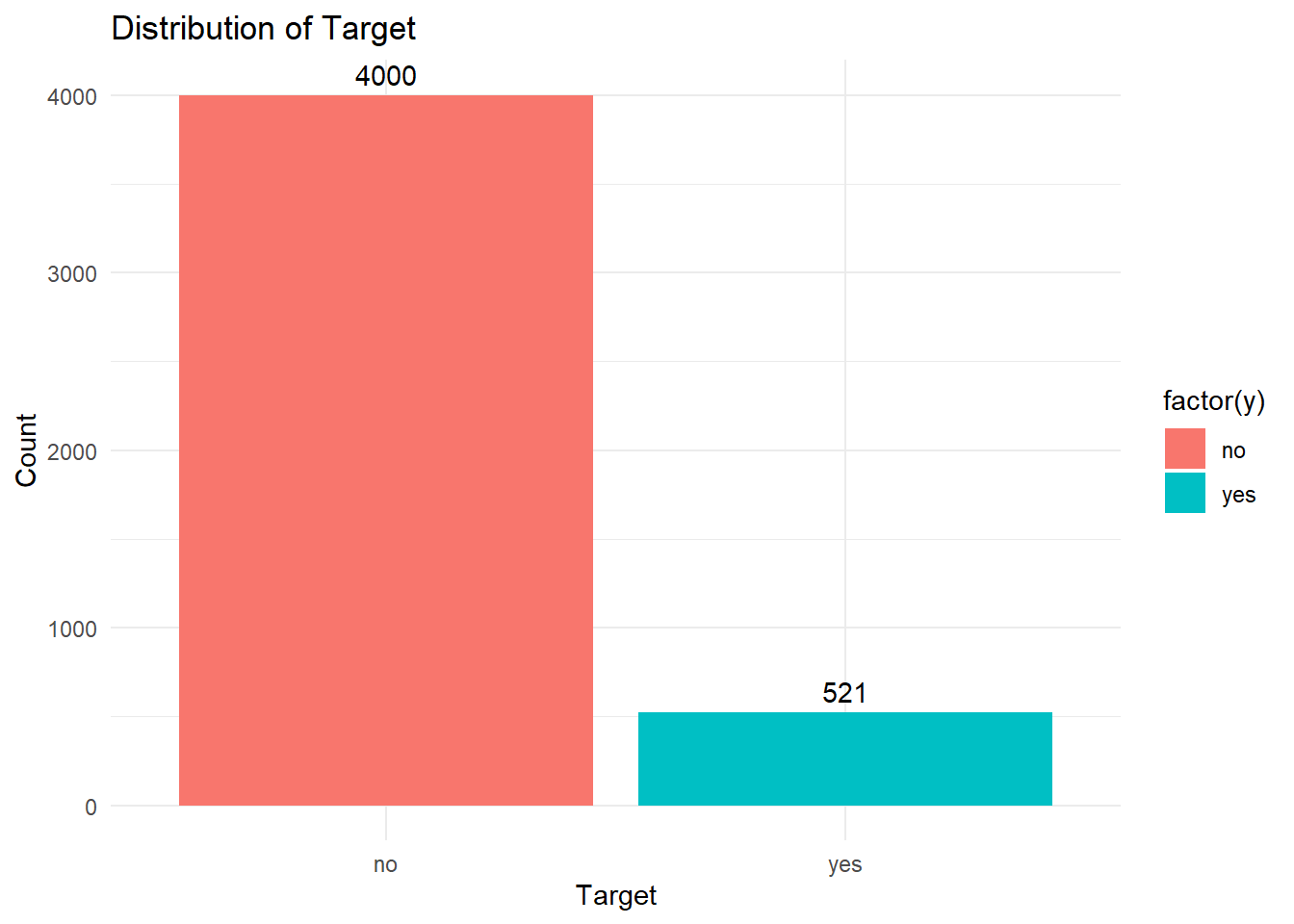
# Data processingdata <- data0 |>select(age,job,marital,education,default, balance,housing,loan,duration, campaign,pdays,previous,poutcome,y)# # Check data type# data %>% str# Convert the variables to categoricaldata$job <-as.factor(data$job)data$marital <-as.factor(data$marital)data$education <-as.factor(data$education)data$default <-as.factor(data$default)data$housing <-as.factor(data$housing)data$loan <-as.factor(data$loan)data$poutcome <-as.factor(data$poutcome)data$y <-as.factor(data$y)# Check the distribution of the outcome yggplot(data, aes(x =factor(y), fill =factor(y))) +geom_bar() +#geom_bar(fill = "purple") +geom_text(stat ="count", aes(label = ..count..), vjust =-0.5)+labs(x ="Target", y ="Count", title ="Distribution of Target") +theme_minimal()
The number of yes are considerably low compared to no. This indicates we have imbalanced class. First we will look at a simple logistic regression.
# To ensure reproducibilityset.seed(55)# Split data into training and testing setind <-sample(1:nrow(data),floor(0.7*nrow(data)),replace =FALSE)# Training datasetdata_train <- data[ind,]# Testing datasetdata_test <- data[-ind,]
# weights:  151
initial  value 1932.835777
iter  10 value 1084.378919
iter  20 value 1008.871476
iter  30 value 1000.762095
iter  40 value 980.193591
iter  50 value 940.441583
iter  60 value 926.854358
iter  70 value 921.815841
iter  80 value 917.811037
iter  90 value 884.518071
iter 100 value 825.223570
iter 110 value 802.825670
iter 120 value 794.840877
iter 130 value 784.739292
iter 140 value 766.855650
iter 150 value 759.677806
iter 160 value 757.825474
iter 170 value 756.109305
iter 180 value 752.439765
iter 190 value 748.184352
iter 200 value 746.727211
final  value 746.727211
stopped after 200 iterations
# Predictionsy_pred_nnet <-predict(model_nnet, data_test, type ="class")# Confusion MatrixconfusionMatrix(data_test$y, as.factor(y_pred_nnet))
Confusion Matrix and Statistics

          Reference
Prediction   no  yes
       no  1158   35
       yes  106   58

               Accuracy : 0.8961
                 95% CI : (0.8786, 0.9118)
    No Information Rate : 0.9315
    P-Value [Acc > NIR] : 1

                  Kappa : 0.3988

 Mcnemar's Test P-Value : 3.745e-09

            Sensitivity : 0.9161
            Specificity : 0.6237
         Pos Pred Value : 0.9707
         Neg Pred Value : 0.3537
             Prevalence : 0.9315
         Detection Rate : 0.8534
   Detection Prevalence : 0.8791
      Balanced Accuracy : 0.7699

       'Positive' Class : no
# Confusion Matrix data framecm_list$neural_network <-confusionMatrix(data_test$y, as.factor(y_pred_nnet))
The accuracy is close to 89.61% which is not bad. Next we will try support vector classification method.
Confusion Matrix and Statistics

          Reference
Prediction   no  yes
       no  1017  176
       yes  147   17

               Accuracy : 0.762
                 95% CI : (0.7384, 0.7844)
    No Information Rate : 0.8578
    P-Value [Acc > NIR] : 1.0000

                  Kappa : -0.0408

 Mcnemar's Test P-Value : 0.1192

            Sensitivity : 0.87371
            Specificity : 0.08808
         Pos Pred Value : 0.85247
         Neg Pred Value : 0.10366
             Prevalence : 0.85777
         Detection Rate : 0.74945
   Detection Prevalence : 0.87915
      Balanced Accuracy : 0.48090

       'Positive' Class : no
# Confusion Matrix data framecm_list$smote_support_vector_classifier <-confusionMatrix(data_test$y, as.factor(y_pred_svc))
The accuracy is close to 89.61% which is not bad. Next we will try some method to deal with imbalanced dataset using the SMOTE (Synthetic Minority Oversampling Technique) method which tries to balance the classes by oversampling from the minority classes. We will try to run all the models based on the over sampled data and compare them.
# SMOTE methodlibrary(ROSE)data_train2 <-ovun.sample(y ~ ., data = data_train,method ="over", N = (nrow(data_train)*3))$data
# weights:  151
initial  value 6672.439994
iter  10 value 5444.151418
iter  20 value 4928.673252
iter  30 value 4668.104777
iter  40 value 4574.222061
iter  50 value 4493.420471
iter  60 value 4331.950671
iter  70 value 4099.714709
iter  80 value 4002.793010
iter  90 value 3980.135694
iter 100 value 3847.275435
iter 110 value 3731.594349
iter 120 value 3678.434483
iter 130 value 3672.812783
iter 140 value 3671.252056
iter 150 value 3665.833513
iter 160 value 3665.133792
iter 170 value 3663.637799
iter 180 value 3659.793664
iter 190 value 3659.407716
iter 200 value 3658.453928
final  value 3658.453928
stopped after 200 iterations
# Predictionsy_pred_nnet2 <-predict(model_nnet2, data_test, type ="class")# Confusion MatrixconfusionMatrix(data_test$y, as.factor(y_pred_nnet2))
Confusion Matrix and Statistics

          Reference
Prediction  no yes
       no  806 387
       yes  25 139

               Accuracy : 0.6964
                 95% CI : (0.6711, 0.7208)
    No Information Rate : 0.6124
    P-Value [Acc > NIR] : 6.596e-11

                  Kappa : 0.268

 Mcnemar's Test P-Value : < 2.2e-16

            Sensitivity : 0.9699
            Specificity : 0.2643
         Pos Pred Value : 0.6756
         Neg Pred Value : 0.8476
             Prevalence : 0.6124
         Detection Rate : 0.5940
   Detection Prevalence : 0.8791
      Balanced Accuracy : 0.6171

       'Positive' Class : no
# Confusion Matrix data framecm_list$smote_neural_network <-confusionMatrix(data_test$y, as.factor(y_pred_nnet2))
Based on accuracy, neural network model on original data is the best and based on the sensitivity (true positive rate), logistic regression on over sampled data is the best.