ML models to predict fuel consumption of cars (MPG) using car information
analysis
R
Author
Aditya Ranade
Published
May 15, 2025
I found this dataset on UCI machine learning repository which gives the dataset regarding the car features along with fuel consumption. The goal is to predict the fuel consumption indicated by the variable mpg based on other features of the car like horespower, displacement, weight, etc. of car. We will compare multiple Machine Learning models for the same.
library(reshape2)library(ggplot2)library(ggh4x)library(ggcorrplot)library(GGally) # for pairs plot using ggplot frameworklibrary(dplyr)library(glmnet)library(knitr)# Get cars data from github repopath <-"https://raw.githubusercontent.com/adityaranade/portfolio/refs/heads/main/cars/autompg.data"data0 <-read.table(path, fill =TRUE, header =FALSE)colnames(data0) <-c("mpg","cylinders","displacement","horsepower","weight","acceleration","model_year","origin","car_name")# Check the type of datadata0 |>str()
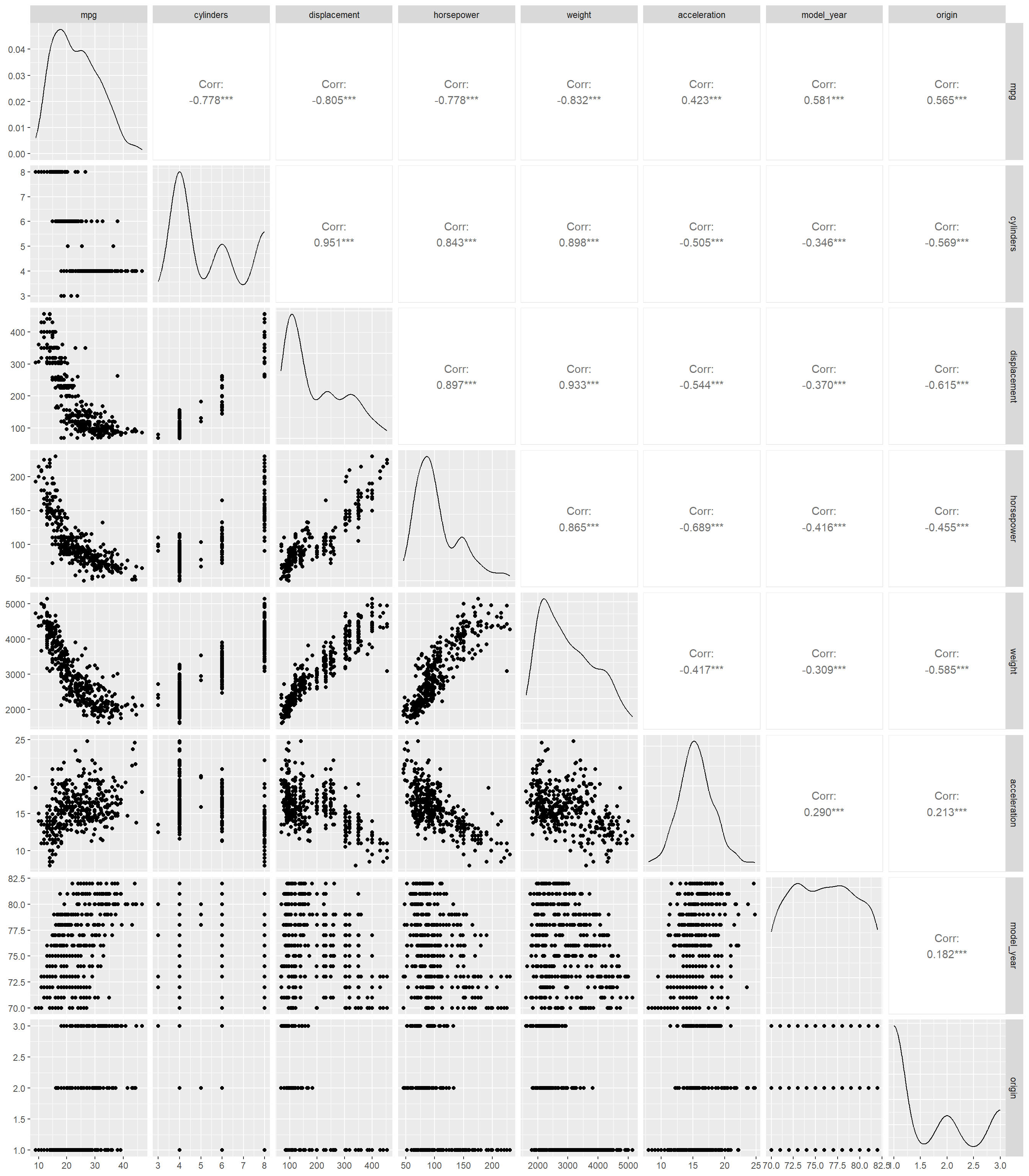
The distributions of the continuous variables on the original scale indicates some non linear relationships between the response variable mpg and the other variables. So we convert the data to log scale and the relationships become close to linear. Hence we will use the data on log scale for predictions. The distribution of the data on the log scale is as follows
# Transform the data to log scale# exclude the last column which is car namedata <- data1[,-ncol(data1)]# Pairs plot between the explanatory variables to # check correlation between each pair of the variablesggpairs(data)
The response variable, mpg is correlated with all the variables which is good. However, the explanatory variables are correlated within themselves which is not a good indication. This indicates there is some multicollinearity. This means two variables give similar information about the response variable. One way to mitigate the effect is to consider the principal components and then use the principal components for the models. Another way is to use some regularization to mitigate the effect of multicollinearity.
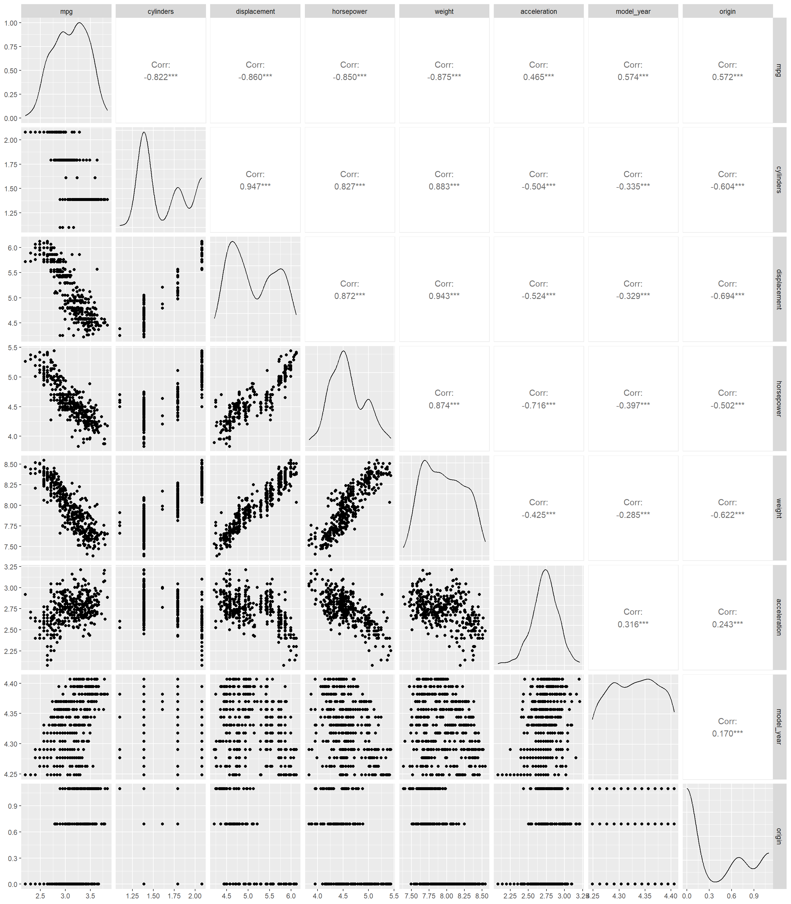
# Transform the data to log scaledata <- data1[,-ncol(data1)] |>log()# Pairs plot between the explanatory variables to # check correlation between each pair of the variablesggpairs(data)
The response variable, mpg is correlated with all the variables which is good. However, the explanatory variables are correlated within themselves which is not a good indication. This indicates there is some multicollinearity. This means two variables give similar information about the response variable. One way to mitigate the effect is to consider the principal components and then use the principal components for the models. Another way is to use some regularization to mitigate the effect of multicollinearity.
# split the data into training and testing dataseed <-23set.seed(seed)ind <-sample(floor(0.8*nrow(data)),replace =FALSE)# Training datasetdata_train <- data[ind,-ncol(data)]# Testing datasetdata_test <- data[-ind,-ncol(data)]
First, we will look at a multiple linear regression model
# Fit a multiple linear regression modelmodel_lm <-glm(mpg ~ ., data = data_train)# Check the summary of the modelmodel_lm |>summary()
Call:
glm(formula = mpg ~ ., data = data_train)

Coefficients:
             Estimate Std. Error t value Pr(>|t|)
(Intercept)   1.49694    0.74566   2.008 0.045573 *
cylinders    -0.06673    0.06434  -1.037 0.300499
displacement -0.04162    0.05169  -0.805 0.421340
horsepower   -0.25381    0.05798  -4.378 1.65e-05 ***
weight       -0.59676    0.08376  -7.125 7.51e-12 ***
acceleration -0.22290    0.06073  -3.670 0.000286 ***
model_year    1.94813    0.16281  11.966  < 2e-16 ***
---
Signif. codes:  0 '***' 0.001 '**' 0.01 '*' 0.05 '.' 0.1 ' ' 1

(Dispersion parameter for gaussian family taken to be 0.01097963)

    Null deviance: 30.4993  on 312  degrees of freedom
Residual deviance:  3.3598  on 306  degrees of freedom
AIC: -514.99

Number of Fisher Scoring iterations: 2
# Prediction on the testing datasety_pred_lm <-predict(model_lm, data_test)# Data frame for observed vs predicteddf_pred_mlr <-data.frame(predicted = y_pred_lm, observed = data_test$mpg)df_pred_mlr$model <-"mlr"# Evaluation metricsrmse_lm <- (data_test$mpg-y_pred_lm) |>mean() |>sqrt()mae_lm <- (data_test$mpg-y_pred_lm) |>abs() |>mean()r2_lm <-1-sum((data_test$mpg - y_pred_lm)^2) /sum((data_test$mpg -mean(data_test$mpg))^2)
Next, we will try the lasso regression which uses the \(L^1\) penalty.
# Lasso regression (L1 penalty)model_l1_cv <-cv.glmnet(as.matrix(data_train[,-1]),as.matrix(data_train[,1]),alpha =0)#find optimal lambda value that minimizes test MSEbest_lambda_l1 <- model_l1_cv$lambda.minbest_lambda_l1
[1] 0.02813141
model_l1 <-glmnet(as.matrix(data_train[,-1]),as.matrix(data_train[,1]),alpha =0, lambda = best_lambda_l1)# Coefficients of the lasso regression model coef(model_l1)
7 x 1 sparse Matrix of class "dgCMatrix"
                     s0
(Intercept)   1.1562832
cylinders    -0.1119517
displacement -0.1014371
horsepower   -0.2373315
weight       -0.4181040
acceleration -0.1806215
model_year    1.7415423
# Prediction on the testing datasety_pred_l1 <-predict(model_l1, s = best_lambda_l1,newx=as.matrix(data_test[,-1]))# Data frame for observed vs predicteddf_pred_l1 <-data.frame(predicted =as.vector(y_pred_l1), observed = data_test$mpg)df_pred_l1$model <-"lasso"# Evaluation metricsrmse_l1 <- (data_test$mpg-y_pred_l1)^2|>mean() |>sqrt()mae_l1 <- (data_test$mpg-y_pred_l1) |>abs() |>mean()r2_l1 <-1-sum((data_test$mpg - y_pred_l1)^2) /sum((data_test$mpg -mean(data_test$mpg))^2)
Next, we will try the ridge regression which uses the \(L^2\) penalty.
# Ridge regression (L2 penalty)model_l2_cv <-cv.glmnet(as.matrix(data_train[,-1]),as.matrix(data_train[,1]),alpha =1)#find optimal lambda value that minimizes test MSEbest_lambda <- model_l2_cv$lambda.minbest_lambda
[1] 0.0006060729
model_l2 <-glmnet(as.matrix(data_train[,-1]),as.matrix(data_train[,1]),alpha =1, lambda = best_lambda)# Coefficients of the ridge regression model coef(model_l2)
7 x 1 sparse Matrix of class "dgCMatrix"
                      s0
(Intercept)   1.53082771
cylinders    -0.06263596
displacement -0.04075770
horsepower   -0.24240969
weight       -0.60741542
acceleration -0.20551149
model_year    1.93416769
# Prediction on the testing datasety_pred_l2 <-predict(model_l2, s = best_lambda,newx=as.matrix(data_test[,-1]))# Data frame for observed vs predicteddf_pred_l2 <-data.frame(predicted =as.vector(y_pred_l2), observed = data_test$mpg)df_pred_l2$model <-"ridge"# Evaluation metricsrmse_l2 <- (data_test$mpg-y_pred_l2)^2|>mean() |>sqrt()mae_l2 <- (data_test$mpg-y_pred_l2) |>abs() |>mean()r2_l2 <-1-sum((data_test$mpg - y_pred_l2)^2) /sum((data_test$mpg -mean(data_test$mpg))^2)
Next, we will try the elastic net regression which is a combination of lasso (\(L^1\) penalty) and ridge (\(L^2\) penalty) regression.
# Elastic netmodel_en_cv <-cv.glmnet(as.matrix(data_train[,-1]),as.matrix(data_train[,1]),alpha =0.5)#find optimal lambda value that minimizes test MSEbest_lambda_en <- model_en_cv$lambda.minbest_lambda_en
# Prediction on the testing datasety_pred_en <-predict(model_en, s = best_lambda_en,newx=as.matrix(data_test[,-1]))# Data frame for observed vs predicteddf_pred_en <-data.frame(predicted =as.vector(y_pred_en), observed = data_test$mpg)df_pred_en$model <-"elastic_net"# Evaluation metricsrmse_en <- (data_test$mpg-y_pred_en)^2|>mean() |>sqrt()mae_en <- (data_test$mpg-y_pred_en) |>abs() |>mean()r2_en <-1-sum((data_test$mpg - y_pred_en)^2) /sum((data_test$mpg -mean(data_test$mpg))^2)
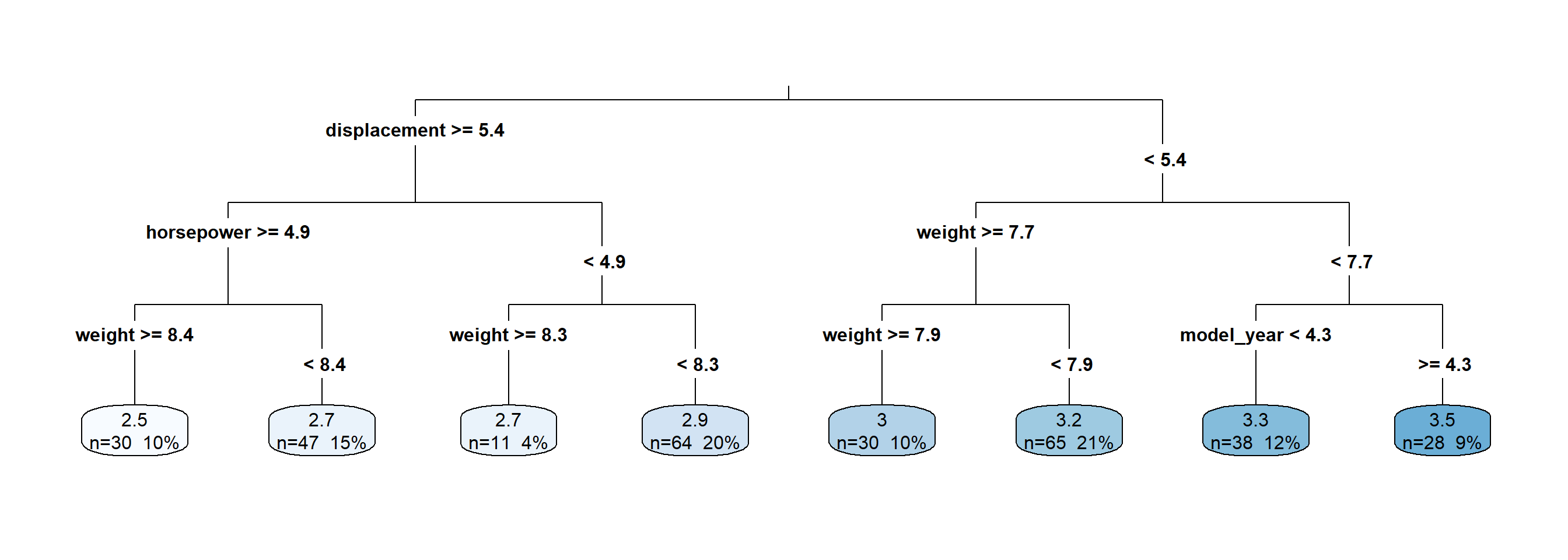
Next, we will try the tree based approach.
# Tree approachlibrary(rpart)library(rpart.plot)# Fit regression treemodel_tree <-rpart(mpg ~ ., data = data_train, method ="anova")# summary(model_tree)# Plotrpart.plot(model_tree, type =3, extra =101, fallen.leaves =TRUE)
y_pred_tree <-predict(model_tree, data_test)# Data frame for observed vs predicteddf_pred_tree <-data.frame(predicted = y_pred_tree, observed = data_test$mpg)df_pred_tree$model <-"tree"# Evaluation metricsrmse_tree <- (data_test$mpg-y_pred_tree)^2|>mean() |>sqrt()mae_tree <- (data_test$mpg-y_pred_tree) |>abs() |>mean()r2_tree <-1-sum((data_test$mpg - y_pred_tree)^2) /sum((data_test$mpg -mean(data_test$mpg))^2)
Next, we will try the random forest approach. In random forest approach, we build multiple trees and then average the predictions of all the trees.
# Random forestlibrary(randomForest)model_rf <-randomForest(mpg ~ ., data = data_train)y_pred_rf <-predict(model_rf, data_test)# Data frame for observed vs predicteddf_pred_rf <-data.frame(predicted = y_pred_rf, observed = data_test$mpg)df_pred_rf$model <-"random_forest"# Evaluation metricsrmse_rf <- (data_test$mpg-y_pred_rf)^2|>mean() |>sqrt()mae_rf <- (data_test$mpg-y_pred_rf) |>abs() |>mean()r2_rf <-1-sum((data_test$mpg - y_pred_rf)^2) /sum((data_test$mpg -mean(data_test$mpg))^2)
Next, we will try the support vector machine (SVM) approach.
library(e1071)model_svm <-svm(mpg ~ ., data = data_train, kernel ="radial", cost =10, gamma =0.1)# Predict on test datay_pred_svm <-predict(model_svm, data_test)# Data frame for observed vs predicteddf_pred_svm <-data.frame(predicted = y_pred_svm, observed = data_test$mpg)df_pred_svm$model <-"svm"# Evaluation metricsrmse_svm <- (data_test$mpg-y_pred_svm)^2|>mean() |>sqrt()mae_svm <- (data_test$mpg-y_pred_svm) |>abs() |>mean()r2_svm <-1-sum((data_test$mpg - y_pred_svm)^2) /sum((data_test$mpg -mean(data_test$mpg))^2)
Next, we will try the extreme gradiant boosting (xgboost) approach.
# xgboostlibrary(xgboost)model_xgb <-xgboost(as.matrix(data_train[,-1]),as.matrix(data_train[,1]),objective ="reg:squarederror",nrounds =100,verbose =0)# Predict on test datay_pred_xgb <-predict(model_xgb, as.matrix(data_test[,-1]))# Data frame for observed vs predicteddf_pred_xgb <-data.frame(predicted = y_pred_xgb, observed = data_test$mpg)df_pred_xgb$model <-"xgboost"# Evaluation metricsrmse_xgb <- (data_test$mpg-y_pred_xgb)^2|>mean() |>sqrt()mae_xgb <- (data_test$mpg-y_pred_xgb) |>abs() |>mean()r2_xgb <-1-sum((data_test$mpg - y_pred_xgb)^2) /sum((data_test$mpg -mean(data_test$mpg))^2)
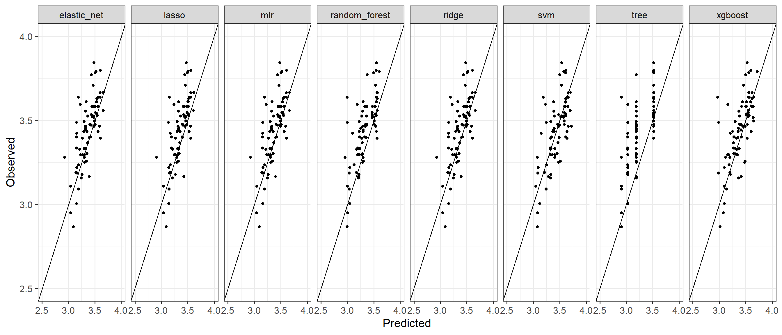
The observed vs. predicted for all the models side by side can be seen in the plot below
# Plot observed vs. predicted for all the modelsdf_pred <-rbind(df_pred_mlr,df_pred_l1,df_pred_l2, df_pred_en, df_pred_tree, df_pred_rf, df_pred_svm,df_pred_xgb)# Create a observed vs. predicted plot combined for all the modelsggplot(df_pred,aes(predicted,observed))+geom_point()+lims(x =c(2.5,4) , y =c(2.5,4))+labs(y ="Observed", x="Predicted")+facet_grid(~model, scales="free")+geom_abline()+theme_bw(base_size =15)
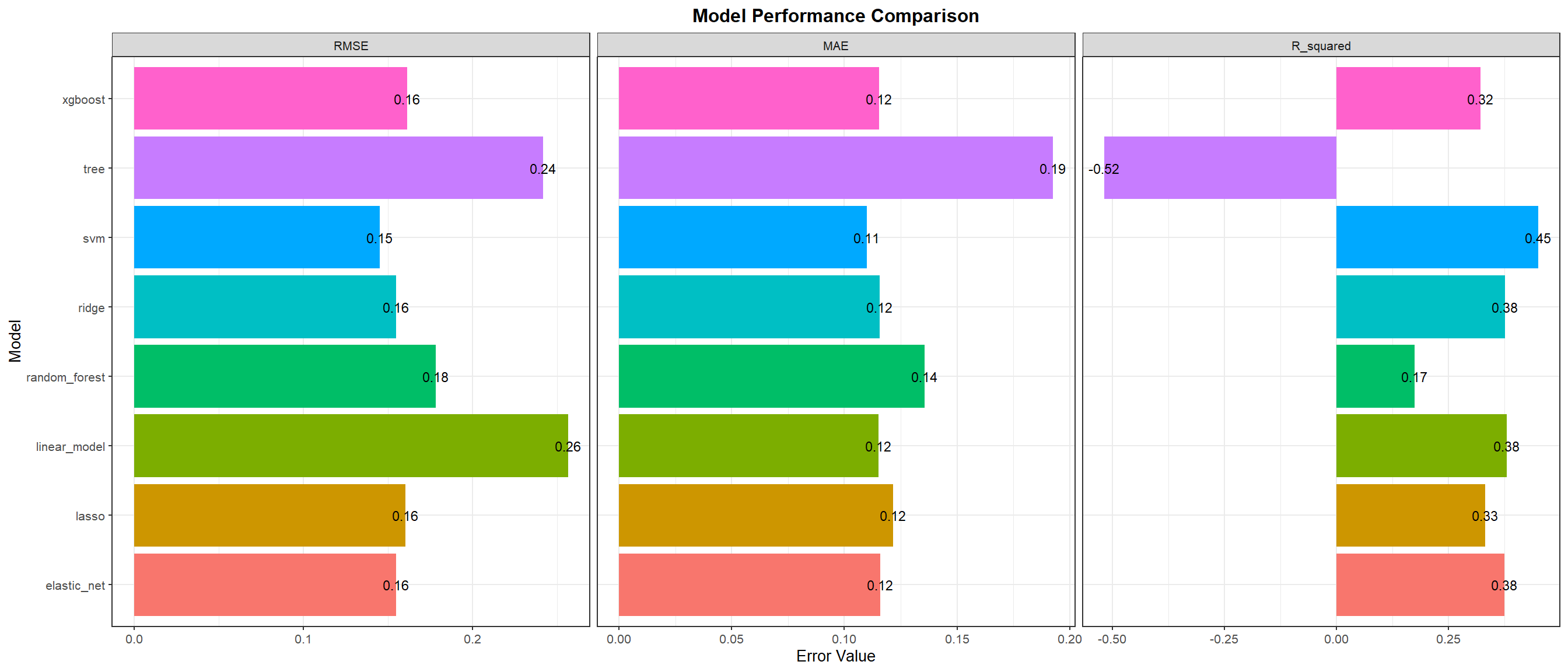
Combined evaluation metrics to compare all the models can be seen in the table below.