Predicting credit approval using binary logistic regression model
analysis
R
Author
Aditya Ranade
Published
March 14, 2025
I found this dataset on UCI machine learning repository which gives the credit approval dataset for a Japanese credit agency. The variable names have been changed to generic names and the factor levels have been changed to general symbols. We will look to build a logistic regression based on the data and try to predict if credit is given or not.
library(reshape2)library(ggplot2)library(dplyr)library(ggh4x)library(cmdstanr)library(bayesplot)library(rstanarm)# Get data from github repopath <-"https://raw.githubusercontent.com/adityaranade/portfolio/refs/heads/main/credit/data/crx.data"data0 <-read.table(path, sep=",")# Data processinghead(data0)
  V1    V2    V3 V4 V5 V6 V7   V8 V9 V10 V11 V12 V13   V14 V15 V16
1  b 30.83 0.000  u  g  w  v 1.25  t   t   1   f   g 00202   0   +
2  a 58.67 4.460  u  g  q  h 3.04  t   t   6   f   g 00043 560   +
3  a 24.50 0.500  u  g  q  h 1.50  t   f   0   f   g 00280 824   +
4  b 27.83 1.540  u  g  w  v 3.75  t   t   5   t   g 00100   3   +
5  b 20.17 5.625  u  g  w  v 1.71  t   f   0   f   s 00120   0   +
6  b 32.08 4.000  u  g  m  v 2.50  t   f   0   t   g 00360   0   +
In this case, we will restrict ourselves to continuous response variables, namely V2, V3, V8, V11 and V15.
# V16 is the response +/- so convert the response to 0 and 1data0$response <-ifelse(data0$V16 =="+",1,ifelse(data0$V16 =="-",0,NA))data0$decision <-ifelse(data0$V16 =="+","credit_granted",ifelse(data0$V16 =="-","credit_not_granted",NA)) # Check the first 6 rows of the datasetdata0 |>head()
  V1    V2    V3 V4 V5 V6 V7   V8 V9 V10 V11 V12 V13   V14 V15 V16 response
1  b 30.83 0.000  u  g  w  v 1.25  t   t   1   f   g 00202   0   +        1
2  a 58.67 4.460  u  g  q  h 3.04  t   t   6   f   g 00043 560   +        1
3  a 24.50 0.500  u  g  q  h 1.50  t   f   0   f   g 00280 824   +        1
4  b 27.83 1.540  u  g  w  v 3.75  t   t   5   t   g 00100   3   +        1
5  b 20.17 5.625  u  g  w  v 1.71  t   f   0   f   s 00120   0   +        1
6  b 32.08 4.000  u  g  m  v 2.50  t   f   0   t   g 00360   0   +        1
        decision
1 credit_granted
2 credit_granted
3 credit_granted
4 credit_granted
5 credit_granted
6 credit_granted
# Convert the data into appropriate factors or numbersdata0$V2 <- data0$V2 |>as.numeric()data0$V3 <- data0$V3 |>as.numeric()data0$V8 <- data0$V8 |>as.numeric()data0$V11 <- data0$V11 |>as.numeric()data0$V15 <- data0$V15 |>as.numeric()# Combine only numerical data along with the responsedata1 <- data0 |> dplyr::select(response,V2,V3,V8,V11,V15)data2 <- data0 |> dplyr::select(decision,V2,V3,V8,V11,V15)# data1 |> str()# Check the number of NA valuessum(is.na(data1))
[1] 12
# Exclude the rows which has NA valuesdata10 <-na.omit(data1)
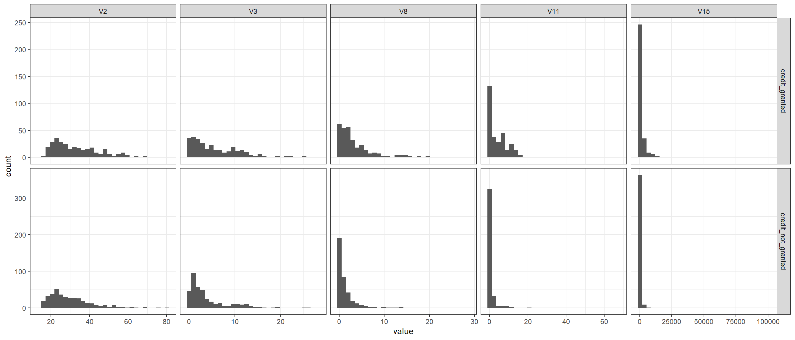
We look at the distribution of the continuous data variables based on if decision variable (credit given / credit not given)
# Data for histogrammelted_data <-melt(na.omit(data2), id="decision")# Plot the histogram of all the variablesggplot(melted_data,aes(value))+geom_histogram(aes(),bins =30)+facet_grid2(decision~variable, scales="free")+theme_bw()
The distribution of the first two variables (V2 and V3) is similar across the decision. So we will exclude these two variables from the model as it is unlikely to have an impact on the decision.
# Exclude V3 and V8 variablesdata <- data10[,-(2:3)]# split the data into training and testing dataseed <-55set.seed(seed)ind <-sample(floor(0.75*nrow(data)),replace =FALSE)# Training datasetdata_train <- data[ind,]# Testing datasetdata_test <- data[-c(ind),]data |>summary()
    response            V8              V11              V15
 Min.   :0.0000   Min.   : 0.000   Min.   : 0.000   Min.   :     0.0
 1st Qu.:0.0000   1st Qu.: 0.165   1st Qu.: 0.000   1st Qu.:     0.0
 Median :0.0000   Median : 1.000   Median : 0.000   Median :     5.0
 Mean   :0.4499   Mean   : 2.209   Mean   : 2.435   Mean   :  1021.2
 3rd Qu.:1.0000   3rd Qu.: 2.574   3rd Qu.: 3.000   3rd Qu.:   395.5
 Max.   :1.0000   Max.   :28.500   Max.   :67.000   Max.   :100000.0
# Read the STAN filefile_stan <-"logistic_regression.stan"# Compile stan modelmodel_stan <-cmdstan_model(stan_file = file_stan,cpp_options =list(stan_threads =TRUE))model_stan$check_syntax()
Now that the model is compiled, we will prepare the data to supply to the model to estimate the parameters based on the training data and make predictions on the testing data.
#Get the data in appropriate form to pass to STAN modelx_train <- data_train[,-1]y_train <- data_train[,1] x_test <- data_test[,-1]y_test <- data_test[,1]x_train <- x_train |>as.matrix()x_test <- x_test |>as.matrix()standata <-list(K =ncol(x_train),N1 =nrow(x_train),X1 = x_train,Y1 = y_train,N2 =nrow(x_test),X2 = x_test,Y2 = y_test)fit_optim <- model_stan$optimize(data = standata,seed = seed,threads =10)
fsum_optim <-as.data.frame(fit_optim$summary())# The optimized parameter would be par_ind <-2:(ncol(x_train)+2)opt_pars <- fsum_optim[par_ind,]opt_pars
# starting value of parametersstart_parameters <-rep(list(list(alpha = opt_pars[1,2],beta = opt_pars[-1,2])),4)# Run the MCMC with optimized values as the starting valuesfit <- model_stan$sample(data = standata,init = start_parameters,seed = seed,iter_warmup =10000,iter_sampling =10000,chains =4,parallel_chains =4,refresh =10000,threads =32,save_warmup =FALSE)
# Save the summaryfsum <-as.data.frame(fit$summary())
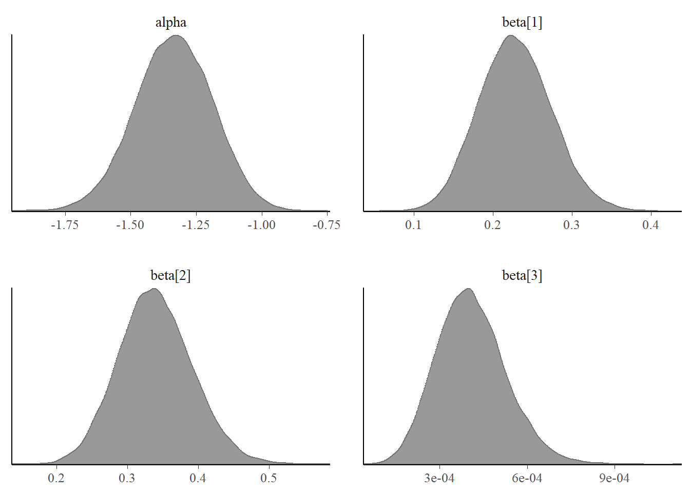
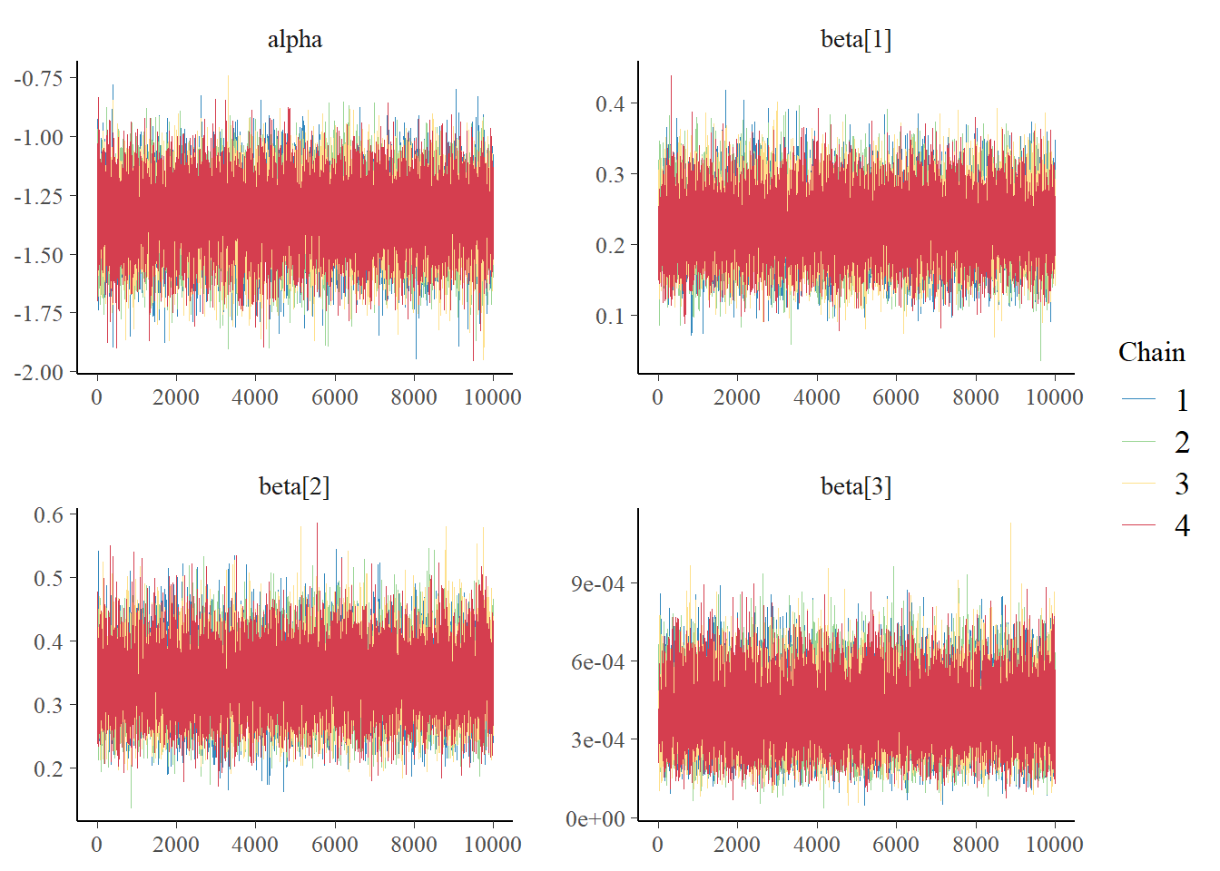
Next we look at the posterior distribution of the parameters and the trace plots. The posterior distribution of the parameters are unimodel and the trace plots indicates a good mix. So no issues with convergence.
# Plot posterior distribution of parametersbayesplot::color_scheme_set("gray")bayesplot::mcmc_dens(fit$draws(c("alpha","beta")))
Now we check the prediction. The STAN model calculates the posterior probability. If the probability is greater than 1, we predict the response to be 1 and 0 otherwise. Based on the predictions, we will generate the confusion matrix.
# Check the predictionspred_ind <- (max(par_ind)+1):(max(par_ind)+length(y_test))# predicted probabilitypred_prob <- fsum[pred_ind,2]pred_outcome <-ifelse(pred_prob>0.5,1,0)# Generate the confusion matrixconf_matrix2 <- caret::confusionMatrix(as.factor(pred_outcome),as.factor(y_test))conf_matrix2
Confusion Matrix and Statistics

          Reference
Prediction   0   1
         0 100  21
         1   9  40

               Accuracy : 0.8235
                 95% CI : (0.7578, 0.8777)
    No Information Rate : 0.6412
    P-Value [Acc > NIR] : 1.358e-07

                  Kappa : 0.5991

 Mcnemar's Test P-Value : 0.04461

            Sensitivity : 0.9174
            Specificity : 0.6557
         Pos Pred Value : 0.8264
         Neg Pred Value : 0.8163
             Prevalence : 0.6412
         Detection Rate : 0.5882
   Detection Prevalence : 0.7118
      Balanced Accuracy : 0.7866

       'Positive' Class : 0
# Accuracyaccuracy <-mean(pred_outcome == y_test)print(paste('Accuracy is ',round(accuracy,4)))
[1] "Accuracy is 0.8235"
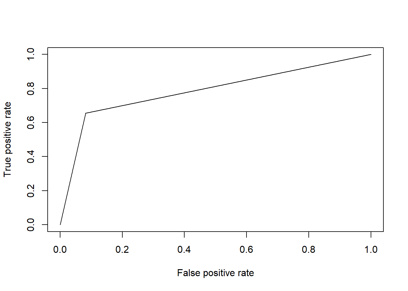
Our model has an accuracy of around 83% which indicates the model is correctly identifying the positive and negative cases in around 83% of the cases. Next, we look at the Receiver Operating Characteristic (ROC) curve. It plots the True Positive Rate (TPR) against the False Positive Rate (FPR). It is the visualization of trade-off between correctly identifying positive cases and incorrectly identifying negative cases as positive. A good model ROC curve which goes from bottom left to top left which means the model is perfectly identifying positive cases and does not identify negatives as positive. On the other hand, a ROC curve which is a straight line from bottom left to to right with slope 1 indicates the model is randomly assigning the positive and negative cases. Our curve is somewhere in between these 2 extreme cases and is decent. The area under the curve (AUC) is around 79% which is also decent.