We use \(\pi\) (pi) in various calculations. \(\pi\) is an irrational number and its value is the ratio of the circumference of a circle to its diameter. In calculations, the commonly accepted value of \(\pi\) is 3.142.. or \(\frac{22}{7}\).
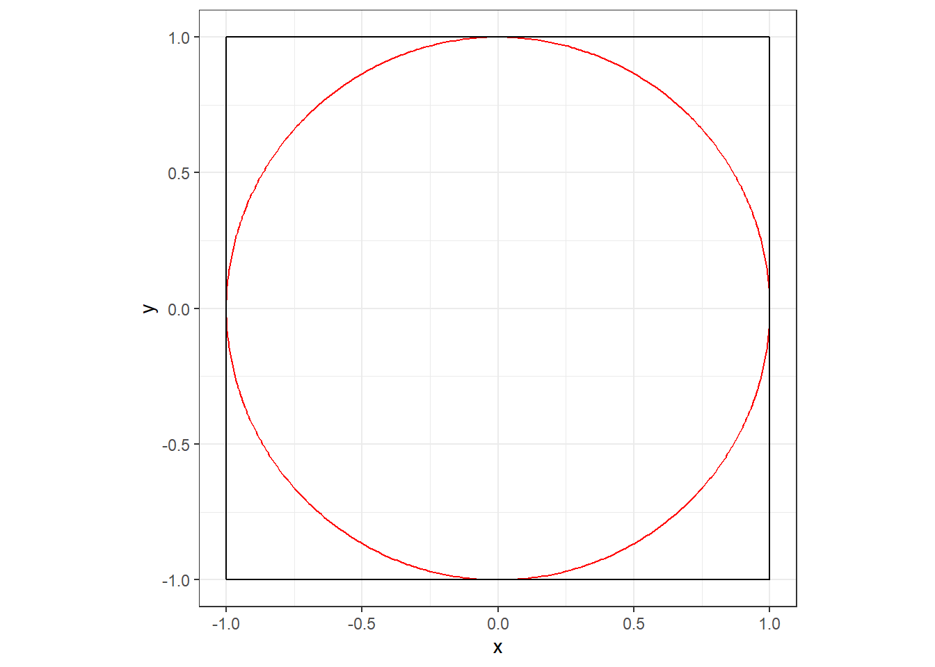
Here, we will attempt to simulate the value of \(\pi\) using monte carlo simulation. We know the area of a circle is \(\pi r^2\) where \(r\) is the radius of the circle and the area of a square is \(s^2\) where \(s\) is the side of the square. Let us have a circle of radius \(r=1\) and bound it in a square whose side is twice of the radius of circle. \(s = 2r\). The figure below shows the circle and square.
Let us look at the ratio of the area of circle to the area of square.
\(\frac{\text{area of circle}}{\text{area of square}} = \frac{\pi * r^2}{s^2} = \frac{\pi * r^2}{(2r)^2} = \frac{\pi}{4}\)
This indicates we can estimate the value of \(\pi\) using the formula
\(\pi = 4 * \frac{\text{area of circle}}{\text{area of square}}\)
Now, we will draw random points in the square and calculate the number of points that fall inside the circle. Then we can estimate the value of \(\pi\) as the ratio of the number of points in the circle divided by the total number of point drawn. Let x and y denote the x and y coordinates respectively. We will draw \(x\) and \(y\) from Uniform(0,1) distribution. The center of the circle is at (1,1). To identify if the point falls in the circle, we will consider the equation of the circle,
\((x-a)^2 + (y-b)^2 = r^2\)
where (a,b) is the center which is (0,0) in our case and r is the radius which is 1 in our case. So the equation simplifies to \(x^2 + y^2 \leq 1\). We will build a function to calculate the value of \(\pi\) as follows
# Function to simulate value of pi where n is
# the number of random points to generate

# Function to simulate value of pi where n is the number of random points to generate
set.seed(33) # to ensure reproducibility

pi_sim <- function(n) {

  x <- runif(n, -1, 1)
  y <- runif(n, -1, 1)

  # Calculate if the point in inside the circle
  inside <- x^2 + y^2 <= 1

  # simulated value of pi
  pi_hat <- 4 * sum(inside)/n

  df <- data.frame(x=x,
                   y=y,
                   inside=inside)

  theta <- seq(0, 2*pi, length.out = 500)
  circle <- data.frame(
  x = cos(theta),
  y = sin(theta))

  p <- ggplot(df, aes(x, y)) +
  geom_point(aes(color = inside), size = 1, alpha = 0.75) +
  geom_path(data = circle, aes(x, y),
            inherit.aes = FALSE,
            linewidth = 0.8,
            color = "black") +
  coord_equal() + theme_bw()+
  scale_color_manual(values = c("FALSE"="red", "TRUE"="blue")) +
  labs(
    title = bquote("Monte Carlo Simulation of " ~ pi ~
               "|" ~ n == .(n) ~
               "|" ~ hat(pi) == .(round(pi_hat,5))),
    x = NULL,
    y = NULL,
    color = "Inside Circle"
    )
  print(p)
}

# Run the function for n = 1000
pi_sim(1000)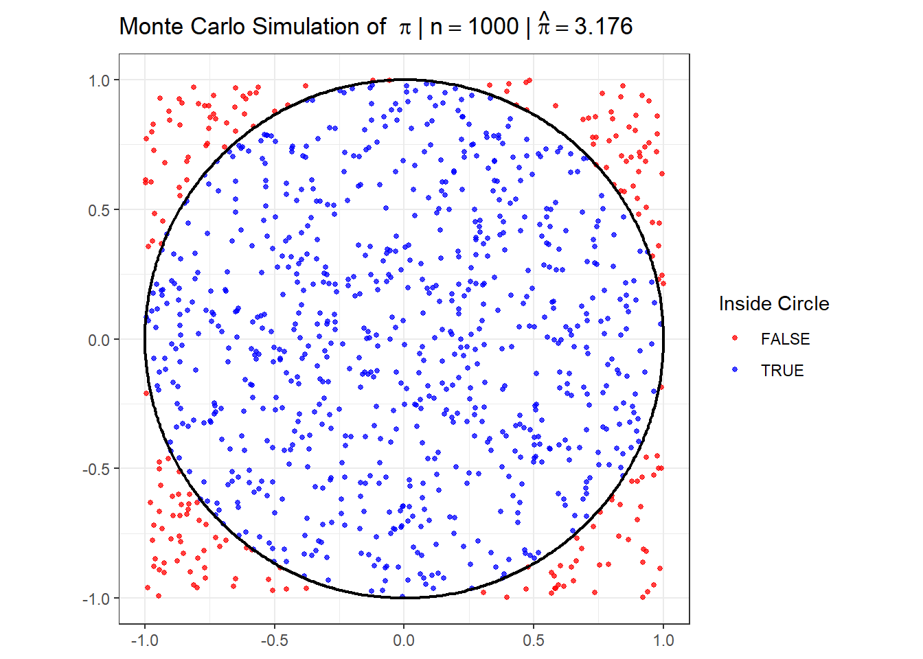
For n = 1000, the simulated value of pi is 3.168. Now, we will try to simulate pi for multiple values of n (500, 1000, 5000, 10000, 20000, 50000)
set.seed(33)

pi_sim_data <- function(n){

  x <- runif(n, -1, 1)
  y <- runif(n, -1, 1)

  inside <- x^2 + y^2 <= 1
  pi_hat <- 4 * mean(inside)

  data.frame(
    x = x,
    y = y,
    inside = inside,
    n = n,
    pi_hat = pi_hat
  )
}

n_vals <- c(1000, 5000, 10000, 20000, 50000, 100000)

df <- do.call(rbind, lapply(n_vals, pi_sim_data))

df$panel <- paste0("n==",
                   df$n,
                   "*','~~hat(pi)==",
                   round(df$pi_hat,5))

df$panel <- factor(df$panel,
                   levels = unique(df$panel[order(df$n)]))

theta <- seq(0, 2*pi, length.out = 500)
circle <- data.frame(
  x = cos(theta),
  y = sin(theta)
)

ggplot(df, aes(x, y)) +

  geom_rect(xmin=-1, xmax=1, ymin=-1, ymax=1,
            fill=NA, color="black") +

  geom_point(aes(color = inside), size=0.7, alpha=0.7) +

  geom_path(data=circle, aes(x,y),
            inherit.aes = FALSE,
            linewidth=0.7) +

  coord_equal() +
  facet_wrap(~panel,
             labeller = label_parsed,
             nrow = 1)+
           # nrow = 1, ncol = length(unique(df$panel)))+
  scale_color_manual(values=c("FALSE"="red","TRUE"="blue")) +
  theme_bw(base_size=15) +
  theme(legend.position = "bottom") +
  labs(title= bquote("Monte Carlo Simulation of " ~ pi),
       x=NULL, y=NULL)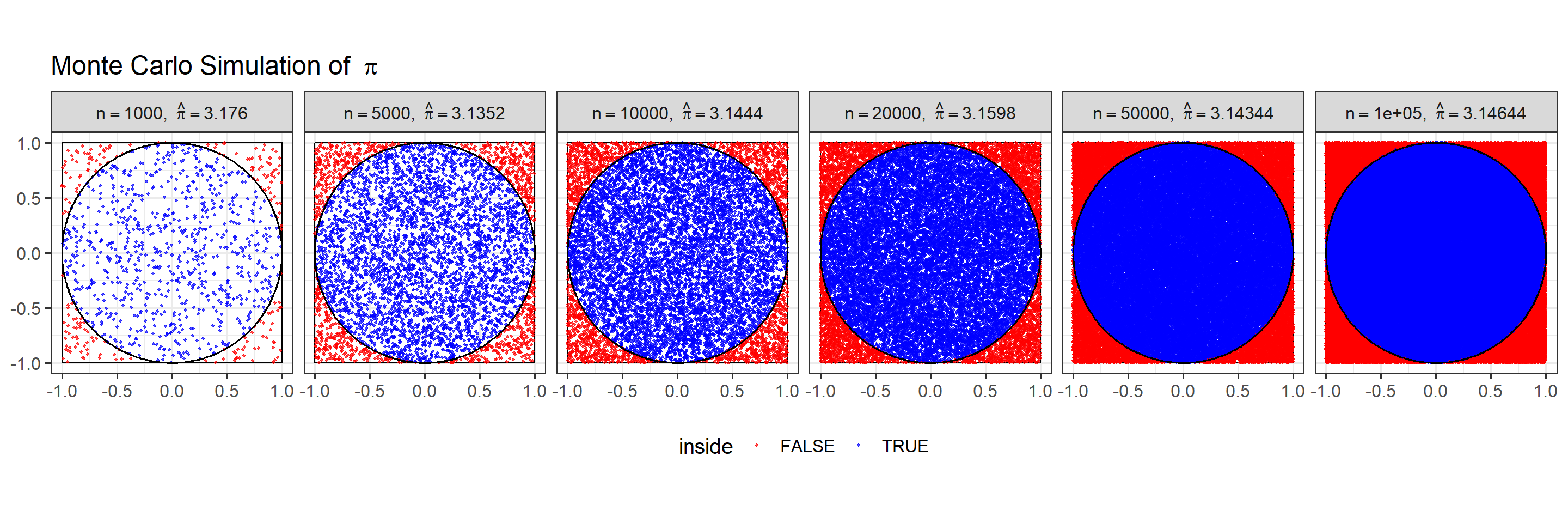
As we can see, the higher the value of n, the estimated value of pi is very close to the accepted value. Now, we will plot the value of pi against the value of points drawn
est_pi <- function(seed = 33, n = 1000) {

  set.seed(seed)

  x <- runif(n, 0, 1)
  y <- runif(n, 0, 1)

  df <- data.frame(x = x, y = y)

  # iteration index
  df$iteration <- seq_len(n)

  # check if inside quarter circle
  df$points_inside_circle <- (df$x^2 + df$y^2) <= 1

  # cumulative estimate of pi
  df$pi_est <- 4 * cumsum(df$points_inside_circle) / df$iteration

  return(df)
}

# generate estimation data for 100,000 points
data <- est_pi(seed = 33, n = 100000)

# Plot
ggplot(data, aes(x = iteration, y = pi_est)) +
  geom_line(color = "blue", linewidth = 0.7) +
  geom_hline(yintercept = pi, linetype = "solid", color = "red") +
  coord_cartesian(ylim = c(3, 3.5)) +
  theme_bw(base_size = 15) +
  labs(
    title = expression("Approximation of " ~ pi),
    x = "Number of points",
    y = expression(~ hat(pi))
  )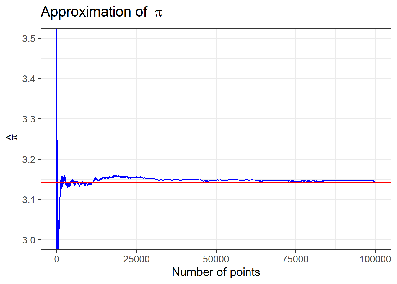
This plot confirms that the higher the value of n, we get really close to the actual value of \(\pi\)