Predicting office room occupancy using binary logistic regression model
analysis
R
Author
Aditya Ranade
Published
April 19, 2025
I found this dataset on UCI machine learning repository which gives the dataset for predicting the room occupancy in office using variables like temperature, humidity, light, carbon-dioxide and humidity ratio. Since the variable of interest is room occupancy, it is binary variable being occupied or not occupied. We will build a logistic regression model to predict the room occupancy using the information. First let us look at the data.
library(reshape2)library(ggplot2)library(dplyr)library(ggh4x)library(GGally)library(pROC)library(glmnet)library(caret)# Get data from github repopath <-"https://raw.githubusercontent.com/adityaranade/portfolio/refs/heads/main/occupancy/occupancy_data.txt"data0 <-read.table(path, sep=",", header =TRUE)# Data processing# Check the type of datadata0 |>str()
'data.frame':   8143 obs. of  7 variables:
 $ date         : chr  "2015-02-04 17:51:00" "2015-02-04 17:51:59" "2015-02-04 17:53:00" "2015-02-04 17:54:00" ...
 $ Temperature  : num  23.2 23.1 23.1 23.1 23.1 ...
 $ Humidity     : num  27.3 27.3 27.2 27.2 27.2 ...
 $ Light        : num  426 430 426 426 426 ...
 $ CO2          : num  721 714 714 708 704 ...
 $ HumidityRatio: num  0.00479 0.00478 0.00478 0.00477 0.00476 ...
 $ Occupancy    : int  1 1 1 1 1 1 1 1 1 1 ...
# Check the rows which do not have any entriessum(is.na(data0)) # No NA values
[1] 0
# Check the first 6 rows of the datasetdata0%>% head
First column is the date which we will ignore. There are no missing values. Occupancy is the binary variable which takes value 0 if the room is not occupied and takes the value 1 if the room is occupied. The explanatory variables are temperature, humidity, light carbon dioxide (CO2) and humidity ratio which are all numerical variables. Next, we will look at the correlation plot which shows the correlation between each pair of the explanatory variables.
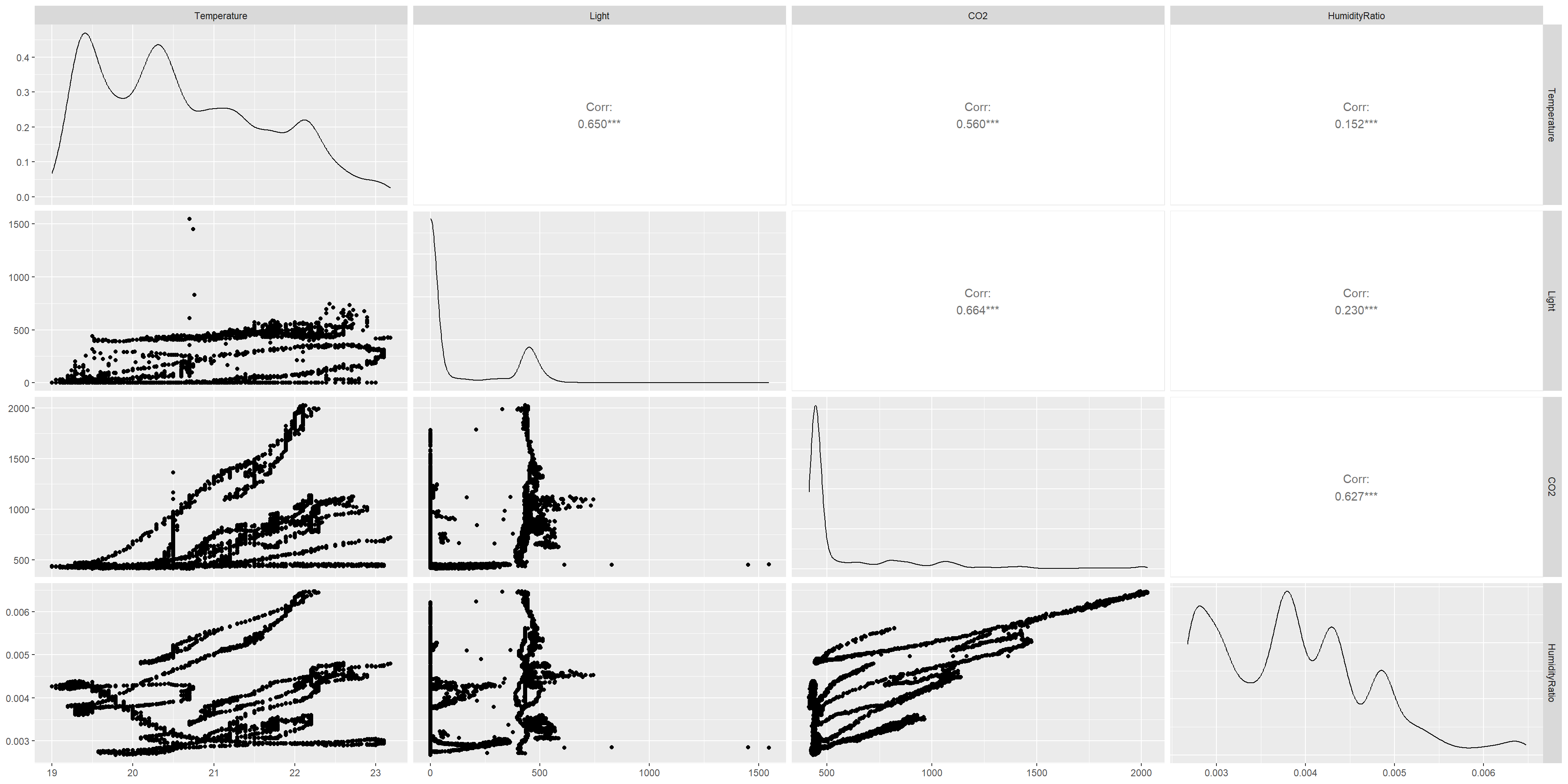
# pairs plot for correlation between every pair of correlationggpairs(data0[,-c(1,3,ncol(data0))]) # exclude the date and binary variable
Humidity and Humidity ratio has high correlation (close to 1). This is on expected lines as humidity ratio is derived from humidity. Now let us look at the distribution of the continuous variables according to occupancy variable.
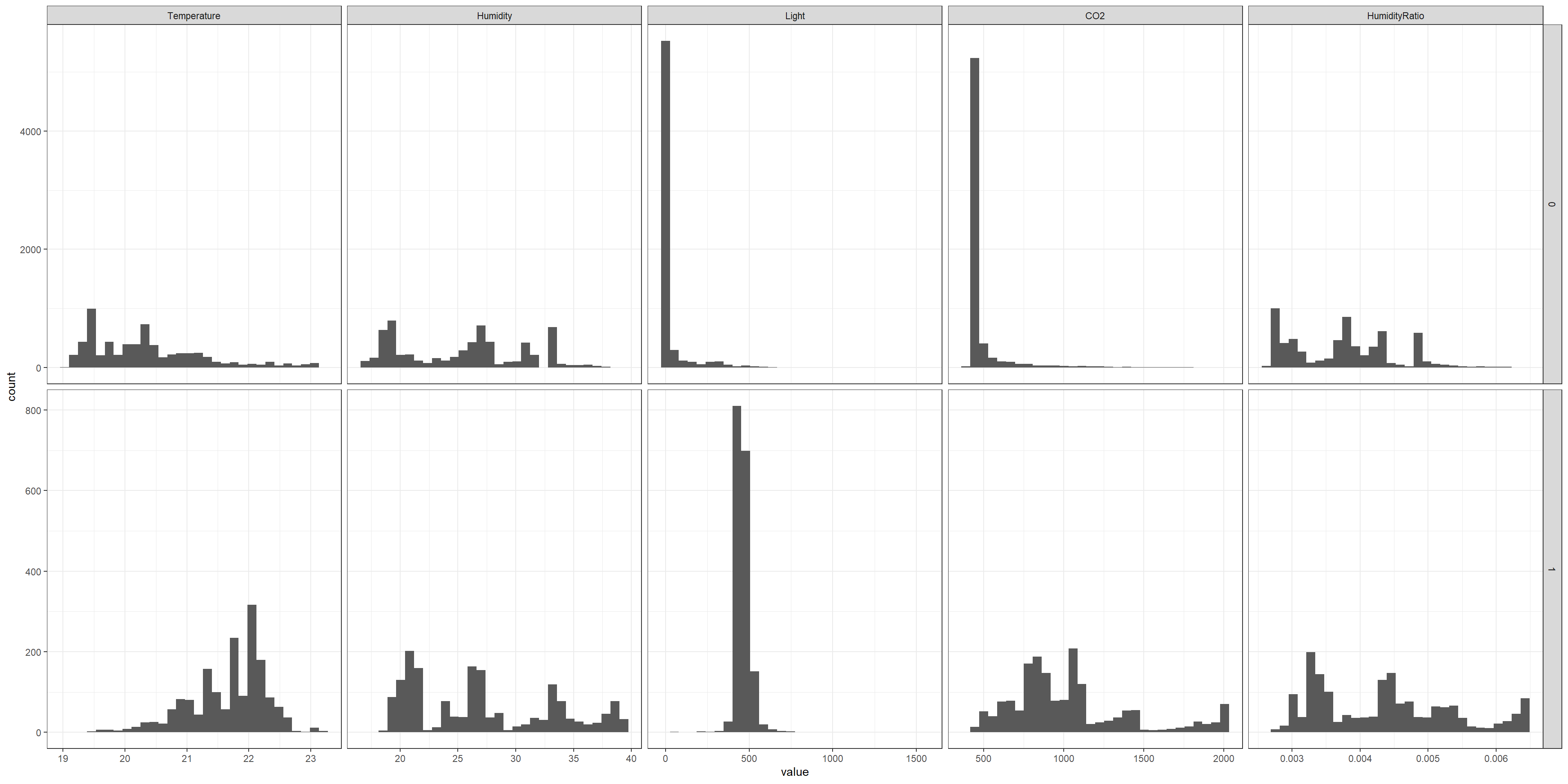
# Data for histogrammelted_data <-melt(na.omit(data0[,-c(1)]), id="Occupancy")# Plot the histogram of all the variablesggplot(melted_data,aes(value))+geom_histogram(aes(),bins =30)+facet_grid2(Occupancy~variable, scales="free")+theme_bw()
We will keep temperature and light in the model as explanatory variable and look to predict the room occupancy using a logistic regression model.
# Select the variables to keep in the modeldata <- data0 |>select(c(Light,HumidityRatio,Occupancy))# split the data into training and testing dataseed <-23set.seed(seed)ind <-sample(floor(0.75*nrow(data)),replace =FALSE)# Training datasetdata_train <- data[ind,]# Testing datasetdata_test <- data[-c(ind),]
# Fit a logistic regression modelmodel <-glm(Occupancy ~ ., data = data_train, family ="binomial") # Check the summary of the modelmodel |>summary()
Call:
glm(formula = Occupancy ~ ., family = "binomial", data = data_train)

Coefficients:
                Estimate Std. Error z value Pr(>|z|)
(Intercept)    -9.489534   0.573068 -16.559  < 2e-16 ***
Light           0.022247   0.001055  21.083  < 2e-16 ***
HumidityRatio 374.622346 141.718350   2.643  0.00821 **
---
Signif. codes:  0 '***' 0.001 '**' 0.01 '*' 0.05 '.' 0.1 ' ' 1

(Dispersion parameter for binomial family taken to be 1)

    Null deviance: 5882.3  on 6106  degrees of freedom
Residual deviance: 1071.6  on 6104  degrees of freedom
AIC: 1077.6

Number of Fisher Scoring iterations: 9
# Prediction probability on the testing datasety_pred_prob <-predict(model, data_test, type ="response")# Prediction class on the testing datasety_pred <-ifelse(y_pred_prob>0.5,1,0)# confusion matrixconf_table <-table(data_test$Occupancy,y_pred)confusionMatrix(conf_table)
Confusion Matrix and Statistics

   y_pred
       0    1
  0 1443    5
  1    3  585

               Accuracy : 0.9961
                 95% CI : (0.9923, 0.9983)
    No Information Rate : 0.7102
    P-Value [Acc > NIR] : <2e-16

                  Kappa : 0.9904

 Mcnemar's Test P-Value : 0.7237

            Sensitivity : 0.9979
            Specificity : 0.9915
         Pos Pred Value : 0.9965
         Neg Pred Value : 0.9949
             Prevalence : 0.7102
         Detection Rate : 0.7087
   Detection Prevalence : 0.7112
      Balanced Accuracy : 0.9947

       'Positive' Class : 0
The misclassification is 8 out of a total of 2036 test cases which is not a bad situation.
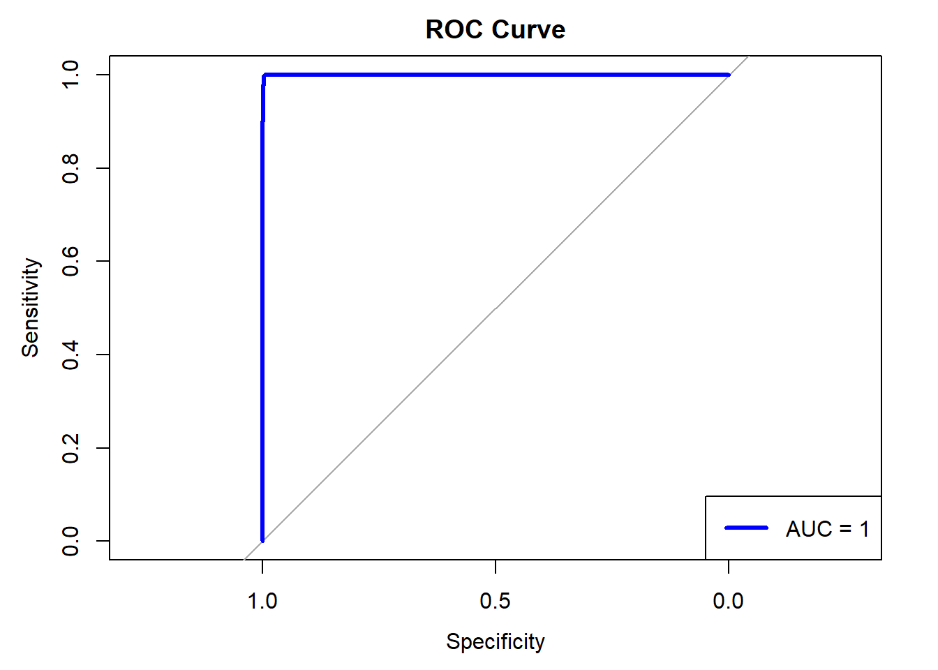
# Compute ROC curveroc_curve <-roc(data_test$Occupancy,as.vector(y_pred_prob))# Calculate AUCauc_value <-auc(roc_curve)# Plot the ROC curveplot(roc_curve, col ="blue", lwd =3, main ="ROC Curve")# Add AUC to the plotlegend("bottomright", legend =paste("AUC =", round(auc_value, 3)), col ="blue", lwd =3)
Misclassification is just around 0.4% on the testing dataset. This is not bad. Also the ROC curve is close to perfect and Area under the curve is also close to 1.