# Load the packages
library(reshape2)
library(ggplot2)
library(ggh4x)
library(ggcorrplot)
library(car) # to calculate the VIF values
library(GGally) # for pairs plot using ggplot frameworkStarbucks is one of the most valued coffee chain in the world. A lot of people like to consume the beverages available at starbucks. But how good are they in terms of the nutritional value?
I found this dataset on Kaggle which gives the nutritional information about their beverages. We will look at the exploratory data analysis first and later try some simple prediction models. First let us access and process the data through R.
# Get starbucks data from github repo
path = "https://raw.githubusercontent.com//adityaranade//portfolio//refs//heads//main//starbucks//starbucks-menu-nutrition-drinks.csv"
data0 <- read.csv(path, header = TRUE)

# Data processing
# change the column names
colnames(data0) <- c("name", "calories", "fat",
                     "carbs", "fiber","protein",
                     "sodium")

# Check the first 6 rows of the dataset
data0 |> head()
name calories fat carbs fiber
1 Cool Lime Starbucks Refreshers™ Beverage 45 0 11 0
2 Ombré Pink Drink - - - -
3 Pink Drink - - - -
4 Strawberry Acai Starbucks Refreshers™ Beverage 80 0 18 1
5 Very Berry Hibiscus Starbucks Refreshers™ Beverage 60 0 14 1
6 Violet Drink - - - -
protein sodium
1 0 10
2 - -
3 - -
4 0 10
5 0 10
6 - -# Check the type of data
data0 |> str()'data.frame': 177 obs. of 7 variables:
$ name : chr "Cool Lime Starbucks Refreshers™ Beverage" "Ombré Pink Drink" "Pink Drink" "Strawberry Acai Starbucks Refreshers™ Beverage" ...
$ calories: chr "45" "-" "-" "80" ...
$ fat : chr "0" "-" "-" "0" ...
$ carbs : chr "11" "-" "-" "18" ...
$ fiber : chr "0" "-" "-" "1" ...
$ protein : chr "0" "-" "-" "0" ...
$ sodium : chr "10" "-" "-" "10" ...The data from second column should be numeric but shows as character. So we first convert it into numeric form and also exclude the rows with missing information
# convert the data to numeric second row onwards
data0$calories <- as.numeric(data0$calories)
data0$fat <- as.numeric(data0$fat)
data0$carbs <- as.numeric(data0$carbs)
data0$fiber <- as.numeric(data0$fiber)
data0$protein <- as.numeric(data0$protein)
data0$sodium <- as.numeric(data0$sodium)

# Check the type of data again
data0 |> str()
'data.frame': 177 obs. of 7 variables:
$ name : chr "Cool Lime Starbucks Refreshers™ Beverage" "Ombré Pink Drink" "Pink Drink" "Strawberry Acai Starbucks Refreshers™ Beverage" ...
$ calories: num 45 NA NA 80 60 NA NA NA 110 0 ...
$ fat : num 0 NA NA 0 0 NA NA NA 0 0 ...
$ carbs : num 11 NA NA 18 14 NA NA NA 28 0 ...
$ fiber : num 0 NA NA 1 1 NA NA NA 0 0 ...
$ protein : num 0 NA NA 0 0 NA NA NA 0 0 ...
$ sodium : num 10 NA NA 10 10 NA NA NA 5 0 ...# Check the rows which do not have any entries
ind.na <- which(is.na(data0[,2]))
length(ind.na) # 85 NA values[1] 85# exclude the rows which has NA values
data <- data0[-ind.na,]Now that we have the data ready, let us look at the histogram each of the variables namely calories, fat, carbs, fiber, protein and sodium
# Data for histogram
melted_data <- melt(data, id.vars="name")

# Plot the histogram of all the variables
ggplot(melted_data,aes(value))+
  # geom_histogram(aes(y = after_stat(density)),bins = 20)+
  geom_histogram(bins = 20)+
  facet_grid2(~variable, scales="free")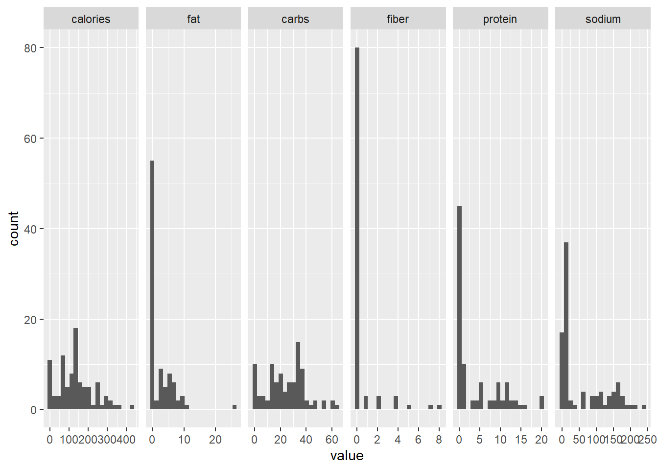
Histogram does not give much information. Let us look at the correlation plot to get an idea of how the variables are correlated with each other.
# correlation plot of all the variables
corr <- round(cor(data[,-1]), 1)
p.mat <- cor_pmat(mtcars) # correlation p-value
# Barring the no significant coefficient
ggcorrplot(corr, hc.order = TRUE,
           type = "lower", p.mat = p.mat)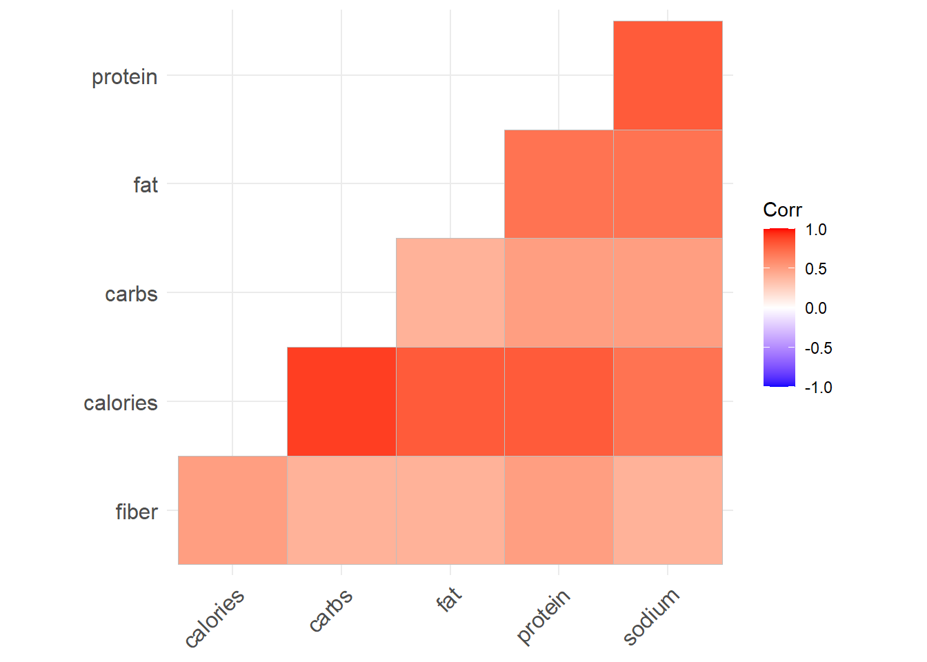
# All positive correlationAll the variables are positively correlated (which indicates when one variable increases, the other variable will increase as well. ) which is not a surprising. Most important part is the correlation of calories with all the other variables are considerably high. Next we look at the pairs plot which will show the bivariate scatter plots as well as the correlation between each variables.
ggpairs(data,columns = 2:ncol(data),
        lower = list(continuous = "smooth"))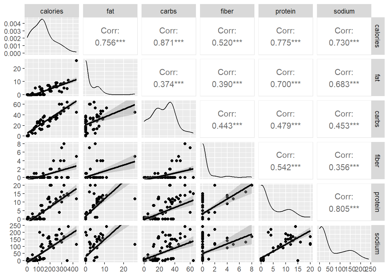
Most of the bivariate scatter plots indicate a linear relationship between the variables. The most important result according to us is the relationship between calories with all the other variables. We can now use the dataset for predictions where we try to predict the calories based o the fat, carb, fiber, protein and sodium content using multiple linear regression.
# split the data into training and testing data
seed <- 23
set.seed(seed)

ind <- sample(floor(0.8*nrow(data)),
              replace = FALSE)

# Training dataset
data_train <- data[ind,-1]
# Testing dataset
data_test <- data[-ind,-1]

# Multiple linear regression using raw data
model <- lm(calories ~ fat + carbs + fiber + protein + sodium, data = data_train)
summary(model)
Call:
lm(formula = calories ~ fat + carbs + fiber + protein + sodium,
    data = data_train)

Residuals:
     Min       1Q   Median       3Q      Max
-14.2823  -1.7523   0.0195   2.1092   8.1259

Coefficients:
            Estimate Std. Error t value Pr(>|t|)
(Intercept)  1.75158    0.94777   1.848   0.0690 .
fat          7.65711    0.25133  30.466  < 2e-16 ***
carbs        3.79744    0.04057  93.599  < 2e-16 ***
fiber        2.51563    0.96443   2.608   0.0112 *
protein      0.75585    0.31682   2.386   0.0199 *
sodium       0.32290    0.03265   9.889 1.01e-14 ***
---
Signif. codes:  0 '***' 0.001 '**' 0.01 '*' 0.05 '.' 0.1 ' ' 1

Residual standard error: 4.131 on 67 degrees of freedom
Multiple R-squared:  0.9976,    Adjusted R-squared:  0.9974
F-statistic:  5493 on 5 and 67 DF,  p-value: < 2.2e-16
# Prediction on the testing dataset
y_pred <- predict(model, data_test)
# Create a observed vs. predicted plot
ggplot(NULL,aes(y_pred,data_test$calories))+geom_point()+
labs(y = "Observed", x="Predicted")+geom_abline()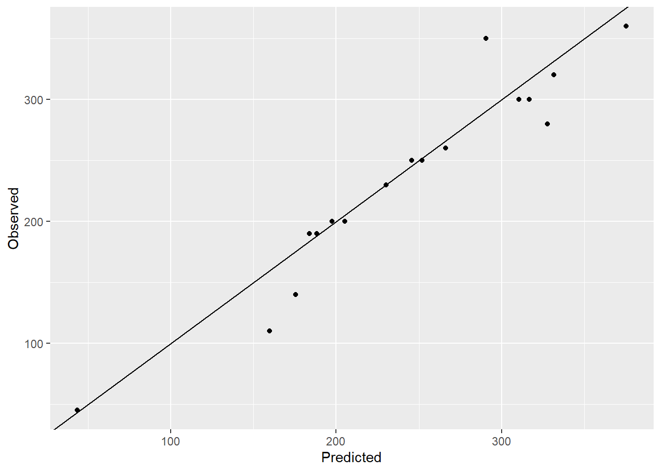
# Calculate RMSE
rmse <- (y_pred-data_test$calories)^2 |> sum() |> sqrt()
rmse
[1] 102.3342# Check the variance inflation factor
vif_values <- vif(model)
vif_values fat carbs fiber protein sodium
3.849325 1.266592 3.382455 10.380709 11.704360 # Check the assumptions of the regression model
# par(mfrow = c(2, 2))
# plot(model)The model is decent with RMSE 102.33 and the observed vs. predicted plot also looks decent. However the variation inflation factor (VIF) value for protein and sodium is higher than 10 which indicates that these two variables are highly correlated with at least one other input variable and hence the variation of these variables is inflated. This might lead to unreliable models. One way to mitigate the multicollinearity problem is to use principal components in place of the correlated variables.
We will create principal components and look how much variation is explained by each of the principal components.
pc <- prcomp(data[,-(1:2)],
             center = TRUE,
             scale. = TRUE)
attributes(pc)
$names
[1] "sdev" "rotation" "center" "scale" "x"
$class
[1] "prcomp"# Check the factor loading of the principal components
print(pc)Standard deviations (1, .., p=5):
[1] 1.7690827 0.8908878 0.7580688 0.5812294 0.4051785
Rotation (n x k) = (5 x 5):
PC1 PC2 PC3 PC4 PC5
fat 0.4610104 0.3810085 0.1092277 0.7933177 0.03190861
carbs 0.3784887 -0.5448572 -0.7329252 0.1443775 -0.04304364
fiber 0.3758452 -0.6263993 0.6433047 -0.0153384 0.22866603
protein 0.5161622 0.1647649 0.1161063 -0.3649765 -0.74815813
sodium 0.4863462 0.3720747 -0.1535201 -0.4651440 0.62056454# Check the summary of the principal components
summary(pc)Importance of components:
PC1 PC2 PC3 PC4 PC5
Standard deviation 1.7691 0.8909 0.7581 0.58123 0.40518
Proportion of Variance 0.6259 0.1587 0.1149 0.06757 0.03283
Cumulative Proportion 0.6259 0.7847 0.8996 0.96717 1.00000The first four principal components explain around 96.72 % of the variation in the data. We will use the first four principal components for the regression model.
data_pc <- cbind(data[,1:2],pc$x)
# training data
data_pc_train <- data_pc[ind,-1]
# testing data
data_pc_test <- data_pc[-ind,-1]

# Multiple linear regression using PC
model_pc <- lm(calories ~ PC1 + PC2 + PC3 + PC4, data = data_pc_train)
summary(model_pc)
Call:
lm(formula = calories ~ PC1 + PC2 + PC3 + PC4, data = data_pc_train)

Residuals:
     Min       1Q   Median       3Q      Max
-15.3780  -1.5028   0.7182   2.2345   7.4206

Coefficients:
            Estimate Std. Error t value Pr(>|t|)
(Intercept) 135.7766     0.5642  240.67   <2e-16 ***
PC1          49.2547     0.3746  131.47   <2e-16 ***
PC2         -12.8205     0.9443  -13.58   <2e-16 ***
PC3         -40.1362     0.9209  -43.59   <2e-16 ***
PC4          22.9143     0.9862   23.23   <2e-16 ***
---
Signif. codes:  0 '***' 0.001 '**' 0.01 '*' 0.05 '.' 0.1 ' ' 1

Residual standard error: 4.442 on 68 degrees of freedom
Multiple R-squared:  0.9971,    Adjusted R-squared:  0.997
F-statistic:  5935 on 4 and 68 DF,  p-value: < 2.2e-16
# Prediction on the testing dataset
y_pred_pc <- predict(model_pc, data_pc_test)
# Create a observed vs. predicted plot
ggplot(NULL,aes(y_pred_pc,data_test$calories))+geom_point()+
labs(y = "Observed", x="Predicted")+geom_abline()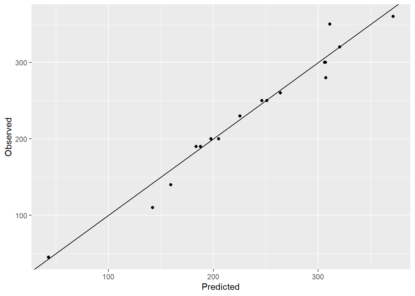
# Calculate RMSE
rmse <- (y_pred_pc-data_pc_test$calories)^2 |> sum() |> sqrt()
rmse
[1] 63.72554# Check the variance inflation factor
vif_values_pc <- vif(model_pc)
vif_values_pc PC1 PC2 PC3 PC4
1.129946 1.471886 1.373721 1.160650 # Check the assumptions of the regression model
# par(mfrow = c(2, 2))
# plot(model_pc)RMSE for the regression model using the first four principal components is 63.73. The variation inflation factor is less than 1.5 for all the principal components. So using less variables with principal components gives much better predictions.