I found this dataset on UCI machine learning repository which gives the dataset related to red and white variants of the Portuguese “Vinho Verde” wine which has physicochemical variables (input) and sensory variables (output) available. Due to privacy, the wine brand, type of grape and selling price is not provided. In this post, we will try to predict the quality based on the physicochemical variables.
library(reshape2)library(ggplot2)library(ggh4x)library(ggcorrplot)library(GGally) # for pairs plot using ggplot framework# Load the datapath <-"https://raw.githubusercontent.com/adityaranade/portfolio/refs/heads/main/wine/winequality-red.csv"data0 <-read.csv(path, header =TRUE)# Data processing# Check the type of datadata0 |>str()
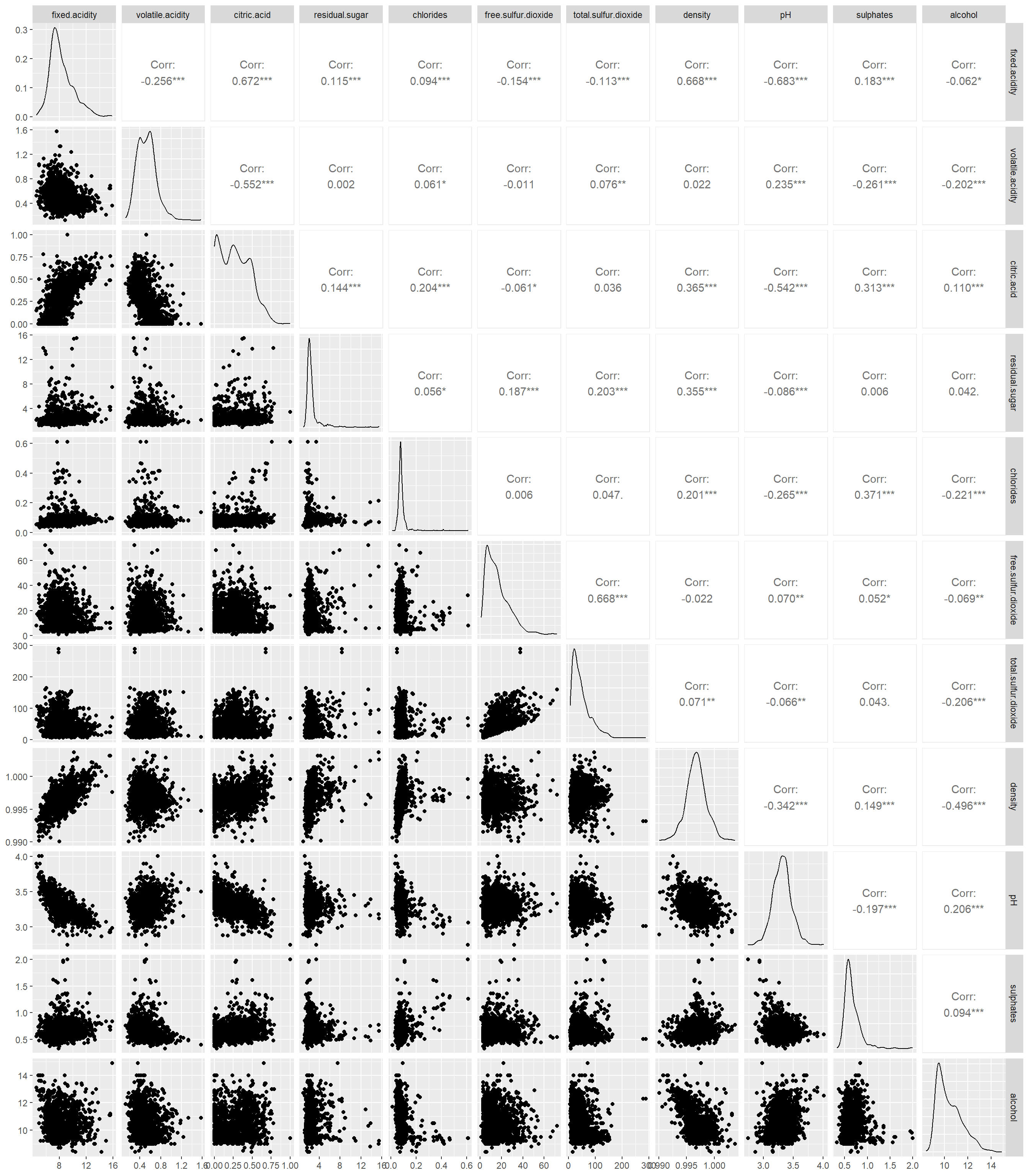
# Pairs plot between the explanatory variables to # check correlation between each pair of the variablesggpairs(data[,-ncol(data)])
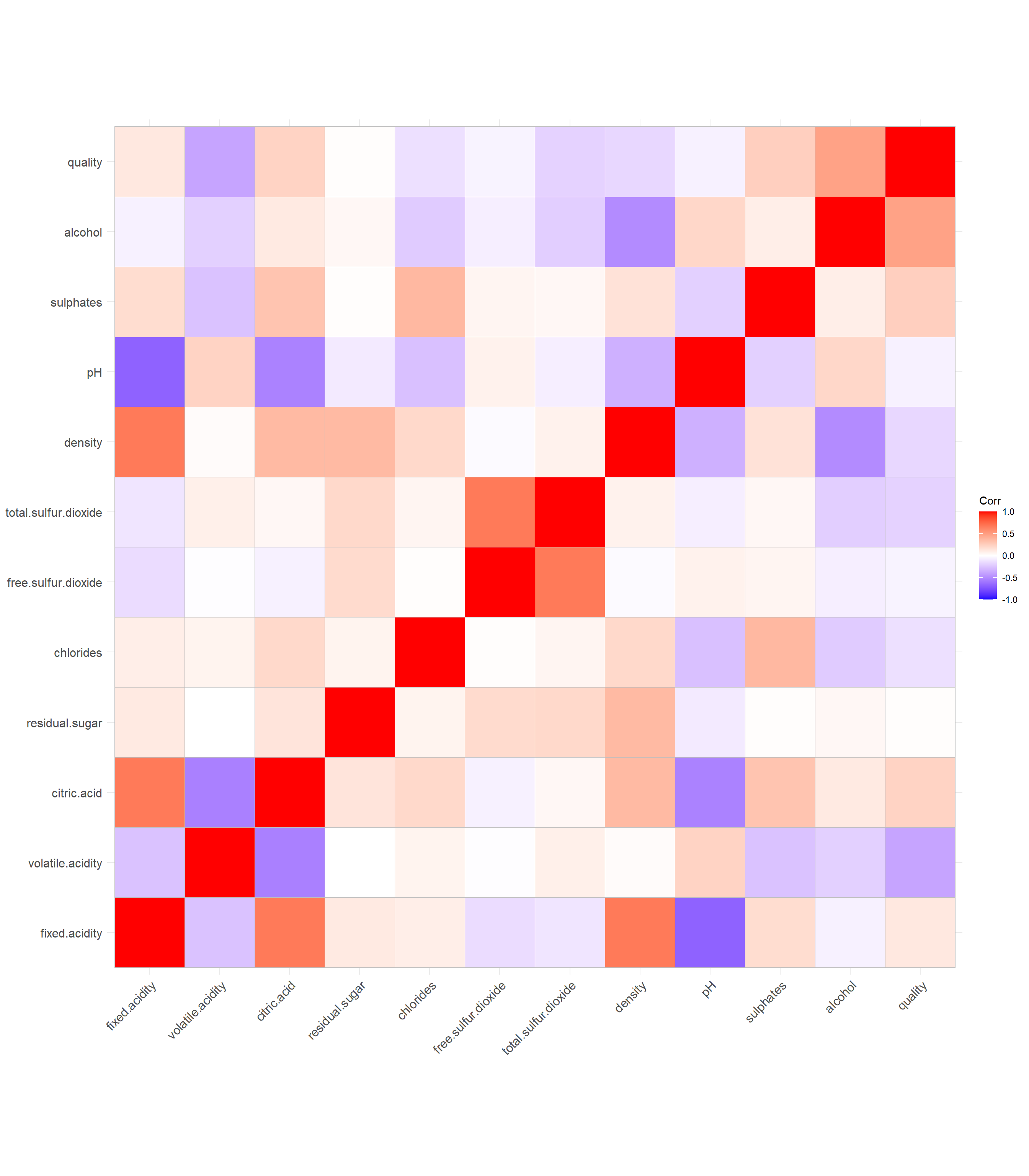
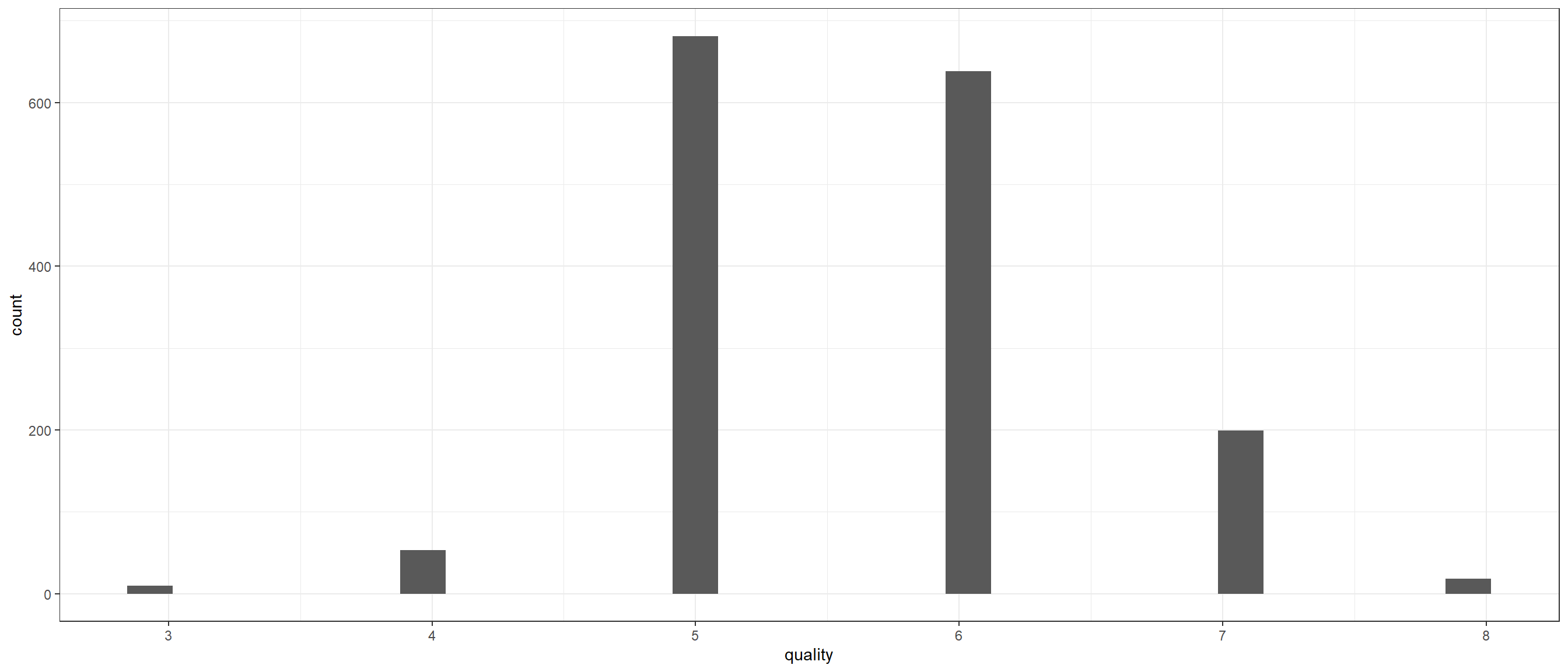
The correlation plot indicates moderate multicolinearity. The histogram of the response variable quality can be seen below. It can be seen most of the entries take the value 5, 6 or 7. Very few entries have value 3, 4 or 8.
# Check the histogram of the response variableggplot(data,aes(quality))+geom_histogram()+theme_bw()
This can be treated as a count data and we can use the Poisson regression. However in Poisson regression, the mean and variance of the response variable quality should be same.
# Check if the mean and variance of response variable is same.# Meandata$quality %>% mean
[1] 5.636023
# Variancedata$quality %>% var
[1] 0.6521684
The mean is considerably greater than variance. Hence Poisson regression model will not work well. An alternative is to use a quasi Poisson model or Negative Binomial model. We will start with a basic multiple linear regression model. First we process the data and standardize all the variables.
# Standardize the data# Scale everything except the response variable (last column)data2 <- datadata2[, -ncol(data)] <-scale(data[, -ncol(data)])# split the data into training and testing dataseed <-23set.seed(seed)ind <-sample(1:nrow(data2),floor(0.8*nrow(data2)),replace =FALSE)# Training datasetdata_train <- data2[ind,] |>as.data.frame()# Testing datasetdata_test <- data2[-ind,] |>as.data.frame()data_test |>dim()
[1] 320 12
Now we run a linear regression model with quality being predicted as a response to volatile acidity, chlorides, total sulfur dioxide, pH, sulphates and alcohol. These variables have been selected after trying multiple combinations of predictor variables. Once we build the model and make predictions, we will round the response variable and make a Predicted vs. actual table. This will help us understand how many correct values were predicted.
# Prediction on the testing datasety_pred <-predict(model, data_test, type ="response")# # Create a observed vs. predicted plot# ggplot(NULL,aes(y_pred,data_test$quality))+geom_point()+# labs(y = "Observed", x="Predicted")+theme_minimal()+geom_abline()table_lm <-table(Predicted =as.factor(round(y_pred)),Actual =as.factor(data_test$quality))table_lm
Since there is some multicolinearity in the data, we can try to use L2 regularization which is also called as ridge regression. This helps shrink the coefficients of the model towards zero.
library(glmnet)
Warning: package 'glmnet' was built under R version 4.4.3
Loading required package: Matrix
Loaded glmnet 4.1-8
#| label: mlr#| echo: true#| warning: false#| include: truemodel_l2_cv <-cv.glmnet(as.matrix(data_train[,-ncol(data_train)]),as.matrix(data_train[,ncol(data_train)]),alpha =1)#find optimal lambda value that minimizes test MSEbest_lambda <- model_l2_cv$lambda.minbest_lambda
# Prediction on the testing datasety_pred_l2 <-predict(model_l2, s = best_lambda,newx=as.matrix(data_test[,-ncol(data_test)]))table_l2 <-table(Predicted =as.factor(round(y_pred_l2)),Actual =as.factor(data_test$quality))table_l2
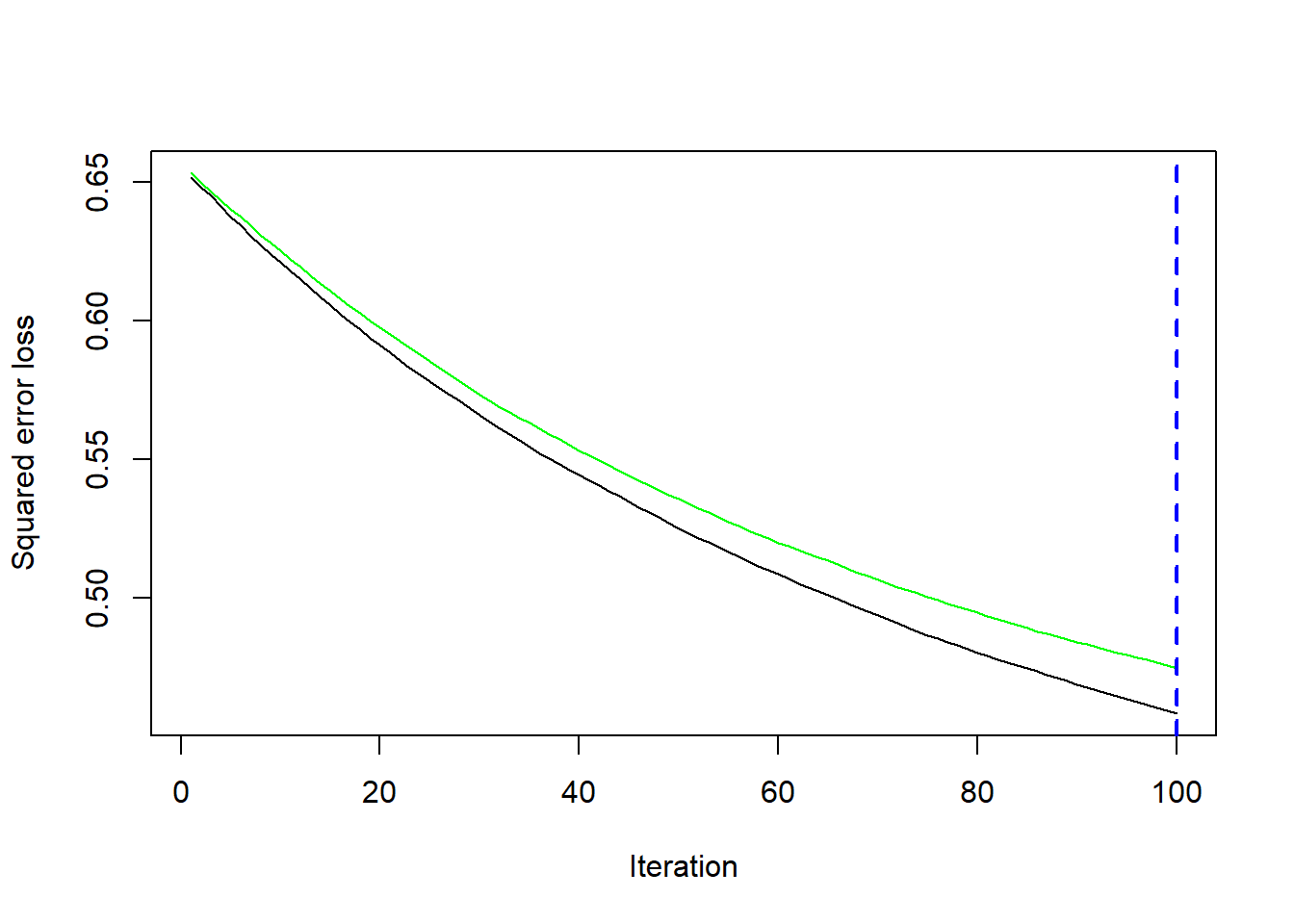
Now, we will try Xgboot (Xtreme Gradient Boosting) model.
# XGBOOSTlibrary(xgboost)# Convert to matrix (xgboost requires the data as matrix or DMatrix format)data_train_matrix <-as.matrix(data_train[,-ncol(data_train)]) target <- data_train[,ncol(data_train)]# Create a DMatrix object (this is how xgboost stores and handles data)dtrain <-xgb.DMatrix(data = data_train_matrix, label = target)params <-list(objective ="reg:squarederror", # Objective function (regression)eta =0.1, # Learning ratemax_depth =6, # Maximum depth of treescolsample_bytree =0.8, # Subsample fraction of featuressubsample =0.8, # Subsample fraction of dataalpha =0.1# L2 regularization)xgb_model <-xgb.train(params = params, data = dtrain, nrounds =100, # Number of boosting rounds (iterations)watchlist =list(train = dtrain), # To monitor the training processprint_every_n =10# Print every 10 iterations)
# Make predictions on the testing datadata_test_matrix <-as.matrix(data_test[,-ncol(data_test)]) predictions <-predict(xgb_model, data_test_matrix)table(round(predictions),data_test$quality)
Based on the multiple models, the Extreme Gradiant Boosting (xgboost) model is able to get the most accuracy in out case. It got the quality correctly for 230 out of 320 cases in the testing data set which translates to an accuracy of around 71.88%.